Regression-style models for parameter estimation in dynamic microsimulation: An empirical performance assessment
- Centre of Methods and Policy Application in the Social Sciences, The University of Auckland, New Zealand
- Article
- Figures and data
-
Jump to
- Abstract
- 1. Introduction
- 2. Review of regresssion-style modelling techniques
- 3. Empirical assessment methods.
- 4. Results
- 5. Discussion
- 6. Conclusion
- 1. Mean absolute differences and standardised mean absolute differences data at each age
- 2. Results from significance tests between models
- 3. TESTING EXOGENEITY OF PREDICTORS
- 4. Results
- References
- Article and author information
Abstract
Microsimulation models seek to represent real-world processes and can generate extensive amounts of synthetic data. The parameters that drive the data generation process are often estimated by statistical models, such as linear regression models. There are many models that could be considered for this purpose. We compare six potential models, discuss the assumptions of these models, and perform an empirical assessment that compares synthetic data simulated from these models with observed data. We chose six regression-style models that can be easily implemented in standard statistical software: an ordinary least squares regression model with a lagged dependent variable, two random effects models (with and without an autoregressive order 1within-unit error structure), a fixed effects model, a hybrid model combining features from both fixed and random effects models, and a dynamic panel model estimated with system generalised method of moments. The criterion for good performance was the proximity of fit of simulated data to the observed data on various characteristics. We found evidence of violated assumptions in our data for all the models but found that, for the majority of data characteristics assessed, all the models produced synthetic data that were a reasonable approximation to the observed data, with some models performing better or worse for particular characteristics. We hope more modellers will consider and test the assumptions of models used for parameter estimation and experiment with different model specifications resulting in higher quality microsimulation models and other research applications.
1. Introduction
Microsimulation models seek to represent real-world processes and can generate extensive amounts of synthetic data. It is desirable that the simulated data reproduce empirical benchmark data. When the characteristics and behaviours of individuals are simulated through time in a dynamic microsimulation, the transition equations are often the coefficients from a statistical regression model of some type. Hence, a key decision in creating a dynamic microsimulation model (DMSM) is the choice of statistical model with which to estimate the parameters of the transition equations.
The choice of estimation technique will, in the first instance, depend on whether a continuous- or discrete-time DMSM is being constructed. In a continuous-time DMSM events can occur at any point in time and thus time-to-event models are the primary statistical estimation technique. In a discrete-time DMSM, which is the focus in this paper, values are simulated or updated in discrete time steps, most often, annually. Discrete-time DMSMs have primarily used dichotomous or categorical variables and transition probabilities have been estimated by constructing tables from available data or using logistic regression models. Continuous variables, especially those where the value of the variable in one time period affects the value in the next time period (i.e. state dependent variables), pose more of a challenge and a range of techniques have been used in this instance. These techniques include a variety of regression models as well as more theoretically driven equations that maximise a utility function (Spataro, 2002; Bianchi, Romanelli, & Vagliasindi, 2005; van Sonsbeek, 2010). Table 1 shows the regression-based techniques that have been used for continuous variables in a number of DMSMs. The choice among these techniques is not simple, yet there been little formal discussion or comparison of regression-style estimation techniques for DMSMs.
Statistical regression techniques used by other dynamic microsimulation models (Table legend).
| OLS regression with an LVD | Random effects | Fixed effects |
|---|---|---|
| MINT3: Earnings of retirees who choose to work, earnings of social security beneficiaries (Toder et al., 2002) | PenSim2: Earnings (Emmerson, Reed, & Shephard, 2004) | MINT1: Earnings (Toder et al., 2002) |
| SVERIGE: Earnings (Rephann & Holm, 2004) | MIDAS: Hours worked, wages (Dekkers et al., 2008) | Income Distribution of the Dutch Elderly: Income (Knoef, Alessie, & Kalwij, 2013) |
| DYNAMOD-2: Earnings (Bækgaard, 2002) | DYNASIM-3: Hours worked, earnings (Favreault & Smith, 2004) | MINT3: Pre-retirement earnings after age 50 (Toder et al., 2002) |
| LifePaths: Hours worked (Wolfson, 1995) | SAGE: Earnings (Zaidi et al., 2009) | |
| MINT3: Non-pension wealth, home equity, non-pension assets (Toder et al., 2002) | ||
| SESIM: Earnings, interest paid, size of loan (Klevmarken & Lindgren, 2008) |
An appropriate statistical modelling technique should be chosen by checking that the data meet the assumptions of the model. Additionally, researchers and modellers need to be aware that the true model is unknown and that the choice of model leads to additional uncertainty in parameter estimates and in predictions. If the chosen model is a poor approximation to the true model, then the error in the simulations may be much greater than that indicated by the standard errors of parameter estimates and the Monte Carlo simulation variability.
The final application of the model should also be taken into account. When constructing a DMSM, one must also consider how the modelling technique will affect the utility of the microsimulation model. It is necessary that the simulated data generated reflect observed reality. If they do not, it is hard to draw meaningful conclusions from the DMSM. One also needs to ensure that the full range of desired scenarios can be performed. The statistical model chosen can affect this.
Comparative assessments between different models (for the estimation of parameters to drive a DMSM) are rare in the literature. We use the development of a discrete-time DMSM to model the trajectory of a birth cohort as an opportunity to assess the performance of six candidate regression-style models in generating continuous data that closely reproduces the empirical data. For this purpose we used an established longitudinal study in a New Zealand city (Fergusson & Horwood, 2001). In our empirical assessment we included techniques that have been used in other DMSMs (as outlined in Table 1), even where fundamental statistical assumptions may have been violated. Our interest is whether the parameter estimates from a given model, are able to inform a DMSM that accurately reproduces empirical observed data, regardless of whether the assumptions of the model are met. Although the assessment performed here is specific to our dataset and the results cannot be generalised to others creating an MSM, we trust that it encourages modellers to experiment with different model specifications and provides ideas on what models to consider and on how a comparison between then can be undertaken.
In what follows, we first review the different techniques, focusing on their various assumptions and implementation in a DMSM. We test the assumptions in our dataset and find evidence of violated assumptions for all the models. We then outline the performance assessment method, before going on to report the results comparing the models on a range of criteria and discuss the findings.
2. Review of regresssion-style modelling techniques
For most continuous variables used in DMSMs, the values for one year depend on, or are related to, the values in the previous year or years; a consistent trajectory across time is usually the reality for a given individual. Hence, with each of the techniques, a key concern is to simulate values over time such that the value simulated for a unit for the current time period takes account of the value that was simulated for that variable in the previous time period.
In choosing which regression techniques to use for the empirical assessment, we started with those commonly used by others for discrete-time DMSMs, these being ordinary least squares regression with a lagged dependent variable (OLS-LDV), random effects (RE) (without an LDV) and fixed effects (FE) (see Table 1). We selected three additional techniques that offered some potential further advantages: an extension of the random effects model with autoregressive within-child errors of the first order (AR(1)), a hybrid model combining features from both econometric fixed effects and random effects models, and a dynamic panel model estimated with the generalised method of moments (GMM). We restricted the estimation techniques we considered to those that could be easily implemented by standard regression software. For each of the models there are a number of assumptions that could be violated resulting in biased coefficients. Below, each model is described and key assumptions are discussed.
To define notation that will be applicable for all the estimation techniques, let us write the general model as
where yi,t is the value of the response variable of the child i at time t, xi,t is a vector of predictors or explanatory variables for child i (which may be constant over time or may be time-variant), μi is the individual effects for child i, and υi,t is the deviation in the response for child i at time t from the mean response for child i. γ is the estimated intercept coefficient (which can be thought of as the grand mean under certain parameterisations of yi,t−1 and xi,t), α is the coefficient for the LDV, and β is the vector of coefficients for the predictors.
2.1 OLS regression with LDV (OLS-LDV)
A standard linear regression model is estimated with OLS that includes, as a predictor variable, the lagged dependent variable (LDV) (the value of the dependent variable in the previous time period). This technique is summarised in Box 1. The LDV is included in order to maintain dynamism in the simulated data; it ensures that the value simulated for this year depends on the value of that variable in the previous year. This is an important feature for state-dependent variables in generating data that mimic observed reality.
A key assumption is that there are no individual effects, that is, after taking into account other predictors, they are zero and all individuals have the same intercept. However, with longitudinal data the individual effects are generally not truly zero and so biased parameter estimates can occur. It is a well-documented phenomenon that the inclusion of an LDV in this manner violates the assumptions on the errors and results in biased estimates (Verbeek, 2008:377–378; Cameron and Trivedi, 2005:763–764).
Summary of OLS regression with a lagged dependent variable (LDV).
| Description of approach: | Standard model with an LDV. |
| Estimation: | Ordinary least squares (OLS) |
| Assumptions on individual effects and errors: | μi = 0, εi,t = υi,t~iid N(0, σ2), Cov(εi,t, xi,t) = 0 |
| Estimates of main effects of time-invariant predictors: | Estimated and included directly in the simulation |
| Implementation in the simulation: | Coefficients (γ, α, and β) applied to the corresponding individual values to get predicted mean for each individual. Random number drawn from normal distribution with mean equal to the predicted mean and standard deviation equal to σ. |
| Other advantages and disadvantages: | Simple to estimate the model and implement in the simulation. |
2.2 Random effects (RE)
Because of the problem of including an LDV as a predictor variable, random effects models have been used to generate parameters for use in a DMSM (see Table 1). In the OLS-LDV technique, the LDV predictor variable gives internal consistency and allows the last time-period’s value to affect the value simulated for the current time-period. In the random effects method, there is no LDV predictor but each individual is assigned an individual effect which they maintain throughout the time-frame of the simulation. An individual’s simulated values oscillate around their own individual trajectory and hence a degree of internal consistency is maintained across the simulated life course of an individual. Previously simulated values do not explicitly affect the current simulated values but the individual effects help generate coherent data values for each individual.
An important assumption is that the individual effects are not correlated with other predictors in the model. This can be tested with a Hausman test (Hausman, 1978) that effectively compares the coefficients from a random effects model with those from a fixed effects model (Green, Kim, & Yoon, 2001).
The standard random effects technique with a variance components error structure assumes that, within an individual, the errors are independent. With continuous variables measured multiple times on the same individual, often this is not the case; we may expect observations measured closer together in time to be more similar than observations measured further apart. Therefore we also considered an extension of the random effects model that does not assume this independence but imposes a correlation structure on the within-person errors. We imposed a simple autoregressive structure of the first order (AR(1)). This model is abbreviated as RE-AR(1). These two variations of the random effects technique are summarised in Boxes 2 and 3.
A major decision when using the random effects method is how to assign the individual effects. Some options for doing this are discussed in Panis (2003), Richiardi (2014), and Richiardi and Poggi (2014). In the empirical work in this paper, Richiardi’s Rank Method (Richiardi, 2014; Richiardi & Poggi, 2014) was used. In this method the differences, for the first year, between the observed and predicted outcomes (the linear predictor not including the individual effect) are ranked across all N units. N values are then simulated from the normal distribution corresponding to the random intercepts and from the normal distribution corresponding to the within-unit errors. These are summed to create the overall error term, (εj,t = o). The overall errors are ranked and then random intercepts are assigned by matching the two sets of rankings.
Summary of random effects variance components technique.
| Description of approach: | Random child intercepts. No LDV included (α = 0). |
| Estimation: | Various options but restricted maximum likelihood (REML) used |
| Assumptions on individual effects and errors: | |
| Estimates of main effects of time-invariant predictors: | Estimated and included directly in the simulation |
| Implementation in the simulation: | As for OLS-LDV except each child assigned an individual effect which is added to the predicted mean |
| Other advantages and disadvantages: | Must decide how to include the individual effects and treat them during scenario testing |
Summary of random effects AR(1) technique.
| Description of approach: | Random child intercepts. No LDV included (a = 0). Within-child errors assumed to have an AR(1) structure. |
| Estimation: | Various options but penalized quasi-likelihood used via the R function glmmPQL. |
| Assumptions on individual effects and errors: | |
| Estimates of main effects of time-invariant predictors: | Estimated and included directly in the simulation |
| Implementation in the simulation: | As for variance components RE, except that the standard deviation of the simulated values is now a random draw from a normal distribution when mean equal to ρυi,t-1 and standard deviation σ. In practice, the error (υi,t) was simulated first and then added to the individual fitted value (which includes the individual effect, μi). This error was saved so that it could be used in simulating the error for the next year. |
| Other advantages and disadvantages: | As for variance components RE, plus more programming required to implement AR errors |
2.3 Fixed effects (FE)
If a significant Hausman test leads to concern about the random effects model (due to the violated assumption of independence between individual effects and other predictor variables), a fixed effects model may appeal. A fixed effects model uses only within-person variation and estimates ‘within’ or ‘fixed’ effects which can be interpreted as the effect if an individual changes on a particular predictor. This is opposed to ‘between’ or ‘cross-sectional’ estimates that are interpreted in terms of the difference between group means (see Goodrich (2006) or Zorn (2001) for further explanation on between and within effects). A fixed effects model can be estimated by including dummy variables for the individuals or by transforming the time-variant variables with a deviation score transformation where, for each individual, the difference is taken between the original values of the variable at each time point and their individual-specific mean. The fixed effects technique is summarised in Box 4.
Simulating data using estimates from a fixed effects model can be performed in the same way as for random effects models, except that, in the assignment of individual effects using the Rank method, instead of drawing values from a normal distribution, values are randomly sampled with replacement from the estimates of the individual effects.
In a fixed effects model the individual effects are regarded as fixed to be estimated (as opposed to random variates). The individual effect represents all the unique time-invariant characteristics of an individual that are not captured by the observed time-variant variables. Since this parameter is estimated in the model, it allows the modeller to say that they have controlled for all time-invariant characteristics of the individuals in the dataset, even those not observed. However, because the individual effects are perfectly collinear with the time-invariant characteristics, no effects will be estimated for any time-invariant predictors.
For time-invariant categorical variables, separate fixed effects models can be fit for the different levels of the variable (e.g. separate FE models for males and females). This then allows the effects of a time-invariant categorical variable to be tested in a scenario in an MSM (either by changing the data values of the time-invariant variable of the simulation units or, if scenarios are performed by modifying parameters, by changing the intercept in the models). This approach is only practical however when there are a small number of time-invariant categorical variables and each variable has only a few categories. Even for the case where there are four time-invariant categorical variables, with, say, three variables having three categories and one having two categories (as is the case in our empirical assessment), the number of models to fit is 54. As well as having the rather cumbersome task of fitting so many models, if the sample size is not extremely large, the number of individuals in most of the cells can become too small to confidently estimate the models.
For continuous variables, fixed effects models pose a serious limitation for MSM because scenarios of the direct effects of these variables cannot be tested. Although interactions with time-invariant variables can be included in the model, this only allows scenarios where the rate of change is modified. To illustrate, an age by time-invariant continuous variable interaction, allows the effect of age on the outcome to change as the value of the continuous variable changes and a scenario to be performed where rate of the change (as the continuous variables changes) is modified. If scenarios are performed by changing the distribution of a time-invariant continuous variable, misleading simulation results can occur even if interactions have been included.
A fixed effects model was employed in the empirical assessment as simulated data can be generated and compared to that from other models, but, due to the limitation of scenario testing for time-invariant variables, fixed effects models may not be a feasible option for all MSMs.
Summary of fixed effects technique.
| Description of approach: | Uses only within child variation to estimate fixed/within effects for time-variant predictors. Run as standard regression but include the child IDs as a set of dummy variables or use deviation scores for time-variant variables and exclude time-invariant variables. No LDV included (α = 0). |
| Estimation: | OLS |
| Assumptions on individual effects and errors: | μi estimated, υi,t~iid N(0, σ2), Cov(μi, xi,t) ≠ 0, Cov(μi, υi,t) = 0 |
| Estimates of main effects of time-invariant predictors: | No estimates of main effects. Can include interactions with time-variant predictors. |
| Implementation in the simulation: | As for random effects. |
| Other advantages and disadvantages: | Does not provide estimates of time-invariant variables which are crucial for a fully functioning DMSM. |
2.4 Hybrid model
The main drawback with the fixed effects model is the inability to estimate the direct effects of time-invariant predictors. A model described in Zorn (2001) and Allison (2005) provides a way to estimate both within/fixed effects for time-variant predictors and also between estimates for time-invariant predictors. Allison calls this model a “hybrid” model and this is how we will refer to it in this paper. Goodrich (2005) also discusses this model and calls it a simultaneous parsed model. Each predictor is decomposed into two variables: a ‘mean variable’, denoted Zi, which contains the individual-specific means over all the time periods (for each individual, the mean is repeated for each time point the variable was observed) and represents the between-person variation and, ‘deviation variables’, denoted , constructed by taking, for each individual, the difference between the original values of the variable at each time point and their individual-specific mean. The deviation variables represent the within-person variation. The model is estimated by fitting a model with random intercepts for each individual and including as predictors the time-invariant variables and both the mean and deviation variables for the time-variant variables. The original (non-decomposed) form of the outcome variable is used. We used a standard variance components error structure. The hybrid technique is summarised in Box 5 and can be represented by the following equation:
In the formulation above Zi represents the time-invariant variables as well as representing the ‘mean variables’ of the time-variant variables.
Implementation of a hybrid model in a DMSM can be performed in the same way as described for the random effects model, except that, when applying the coefficients only the estimates from the time-invariant and the deviation variables are used (that is, the estimates from the ‘mean variables’ that are created from the time-variant variables are not used).
Summary of hybrid technique.
| Description of approach: | Estimates fixed effects for time-variant predictors and crosssectional effects for time-invariant predictors. Each predictor decomposed into between-unit variation, Zi, (repeated individual-specific means for each time point) and within-unit variation, (the difference between the raw value and Zi). Model estimated with the outcome in the original form and including the time-invariant predictors, Zi, , and random individual effects. No LDV included. |
| Estimation: | Restricted Maximum Likelihood (REML) |
| Assumptions on individual effects and errors: | μi~iid N(0, ), υi,t~iid N(0, σ2), by construction Cov(μi, ) = 0 (so is not strictly an assumption), Cov(μi, υi,t) = 0, Cov(zi, υi,t) = 0 |
| Estimates of main effects of time-invariant predictors: | Estimated and included directly in the simulation |
| Implementation in the simulation: | As for random effects. For time-invariant variables, the fixed (‘within’) effects are used; the ‘between’ effects of these variables are not used. |
| Other advantages and disadvantages: | Provides fixed effects estimates and main effects for time-invariant variables. Standard errors not correct. |
2.5 Dynamic panel model (DPM) estimated with the generalised method of moments (GMM)
Because the LDV is endogenous (correlated with the errors) including it when using the previous techniques violates assumptions and results in biased parameter estimates. The use of instrumental variable techniques is required for consistent estimation when an LDV is included in the model (Verbeek, 2008:378; Cameron & Trivedi, 2005:765). The simplest way to do this is to use the Anderson-Hsiao levels estimator (Anderson & Hsiao, 1982), a two-stage least squares approach. This uses the second lag of the outcome variable as the instrument for the LDV. More lags can be used as instruments in this approach, but as more lags are used, the available sample size for fitting the model decreases.
The two-stage least squares approach also assumes that the errors are independent and homoscedastic. This is most likely not the case with panel data. We can move to Generalised Method of Moments (GMM) estimators (Hansen, 1982) to overcome these problems. Two broad categories of GMM dynamic panel estimators are difference GMM and system GMM. These techniques are summarised in Boxes 6 and 7 and more in-depth discussions of these estimators can be found in Roodman (2009b) and Bond (2002).
Difference GMM transforms all predictors, usually by differencing and then uses the GMM with lags of the predictors used as instruments (Arellano & Bond, 1991). Different instruments are valid depending on the assumptions that can be made about the correlations between the predictors and the within-child errors (see Bond, 2002). Since this technique estimates an equation in differences, it does not give estimates for time-invariant variables. This means that difference GMM has the same limitations as the fixed effects approach for the scenarios that can be tested in a DMSM.
System GMM (Arellano & Bover, 1995; Blundell & Bond, 1998) does provide estimates for time-invariant variables and so in our empirical comparison we used this approach. This is possible by making an additional assumption that allows another set of instruments to be used for an equation in levels (as opposed to the equation in differences). The lagged values used as instruments for the equation in differences are transformed (e.g. by differencing) to make them exogenous to the individual effects. System GMM estimates parameters using a system of these two sets of moment conditions. The additional instruments can dramatically improve efficiency over difference GMM estimation.
The assumption made for these additional instruments to be valid is that the first differences of the instruments are uncorrelated with the individual effects. This is equivalent to a stationarity assumption for the initial conditions, specifically, that the deviations from the individual long-run means, at the first year, are not related to the individual effects. This assumption can be tested with a Difference in Sargan test. For more on this assumption see Blundell and Bond (1998), Roodman (Roodman, 2009b), and Roodman (2009a).
Summary of difference GMM dynamic panel model.
| Description of LDV included. Uses instrumental variables to deal with the approach: | endogeneity of the LDV and any other predictors. The predictors are transformed (by the first-difference or orthogonal deviations transformation) and then instrumented with lagged levels of the original predictors. |
| Estimation: | Generalised method of moments (GMM) |
| Assumptions on individual effects and errors: | Cov(yi1, υi,t) = 0 (initial conditions predetermined), Cov(yi1, μi) ≠ 0, Cov(μi, xi,t) ≠ 0, xi,t allowed to be correlated with υi,t and earlier errors but not subsequent errors. |
| Estimates of main effects of time-invariant predictors: | No estimates provided |
| Implementation in the simulation: | Change simulated and added to previous value. Estimates applied to the change in the predictors from last time-period. |
| Other advantages and disadvantages: | Complex estimator with many options |
Summary of system GMM dynamic panel model.
| Description of approach: | As for difference GMM DPM but a second ‘levels’ equation is included to form a system of equations. The variables in the levels equation are instrumented with their own first differences. |
| Estimation: | Generalised method of moments (GMM) |
| Assumptions on individual effects and errors: | As for difference GMM, plus Cov(μi, Δwi,t = 0, where w is any instrumenting variable (either x or y) |
| Estimates of main effects of time-invariant predictors: | Estimated and included directly in the simulation |
| Implementation in the simulation: | As for OLS regression with an LDV. |
| Other advantages and disadvantages: | Complex estimator with many options, hard to meet additional assumption |
3. Empirical assessment methods.
The OLS-LDV, random effects, fixed effects, hybrid and dynamic panel system GMM models were compared on their performance in generating simulated values designed to reproduce empirical data.
The assessment of the statistical models for generating synthetic data in a DMSM will be illustrated in the context of the project Modelling the Early Life Course (MELC) (Milne et al., 2014). MELC is a discrete-time cohort micro-simulation, starting with a cohort at birth and ageing the individuals year-by-year. It simulates from birth to age 13 and assesses the influence of child, parental, and family factors on various outcomes. Time-variant attributes are updated at each year and no new individuals enter or leave as the simulation progresses through time. The primary dataset used to estimate parameters for the MELC micro-simulation was longitudinal data from the Christchurch Health and Development Study (CHDS) (Fergusson & Horwood, 2001). This dataset was used to test and illustrate the statistical models assessed. The CHDS cohort consists of children born in 1977 in Christchurch, New Zealand. The original birth cohort consisted of 1265 children, however we only used the data collected annually from ages 8 to 13 (as these were the years for which our outcome variable for the empirical assessment, reading score, were collected). By age 8 there were 1171 children remaining in the cohort; this remained relatively stable over time with 1172 children at age 9, 1067 at age 10, 1073 at ages 11, 12, and 13.
One state-dependent continuous outcome variable was chosen for this empirical work: the child’s performance on the BURT reading test (Gilmore, Croft, & Reid, 1981). Scores can range from 0 to 110 and the version of the test was taken every year from ages 8 to 13. It was important to choose a state-dependent variable for the empirical comparison as the within-person consistency or dynamism is a key aspect of the synthetic data to assess. Reading score is state-dependent or dynamic in the sense that, for an individual, their level of reading ability in the current year is influenced by their reading ability in the previous year.
Predictors used in the regression models.
| Variable | Categories/description |
|---|---|
| Time-invariant Predictors | Values available only at the child’s birth |
| Gender | Male; Female |
| Mother’s education | No formal qualifications; Secondary qualification; Tertiary qualification |
| Father’s education | No formal qualifications, Secondary qualification; Tertiary qualification |
| Family’s socio-economic position | Semi-skilled, Unskilled, unemployed; Clerical, technical, skilled; Professional, managerial |
| Based on the Elley-Irving scale (Elley & Irving, 1976) | |
| Breast-feeding | Duration in months |
| Time-variant Predictors | Values available at each year |
| LDV | The lagged dependent variable; The value of the reading score at the previous year |
| Child’s age | 8 to 13 years |
| Mother’s hours worked | The average number of hours of paid work performed per week by the mother/mother figure |
| Home ownership | Owned or mortgaged; Rented |
| Father’s smoking | The average number of cigarettes smoked per day by the father/father figure |
For each model the same set of predictor variables was used for consistency (listed in Table 2). Quadratic terms of the LDV and age were included where possible, in addition to the linear terms, since the relationship between both the LDV and reading score and between age and reading score was found to be curved. In the OLS-LDV and dynamic panel models, quadratic terms were included for both the LDV and age. In the random effects, fixed effects, and hybrid models, quadratic effects were included for age only.
A cross-validation method was used to test each model. The dataset was randomly split in two, while at the same time ensuring that no data of any individual child was divided between the two datasets. The two datasets were, as much as possible, of equal sizes. The ‘training’ dataset was used to estimate model coefficients. The coefficient estimates from the training dataset were applied to observed data values in the ‘testing’ dataset to generate a set of simulated data. For each set of coefficients (and its accompanying testing dataset), 1000 runs of the simulation were performed with each run producing a set of simulated data from which a series of summary statistics were obtained.
Thirty cross validations were performed. The overall cross-validation process is represented visually in Figure 1. For simplicity, the figure only makes reference to taking a single mean from a simulated dataset and the absolute difference between a simulated and observed mean. The mean could be replaced with any set of statistics such as mean reading scores by a second variable or the percentiles of the reading scores. The statistics (assessment measures) used are described in the ‘Assessment Measures’ section below. Figure 1 shows the process for only one model. The process was repeated for each model but the training and testing datasets were not re-created. The same set of training and testing datasets were used for the assessment of each statistical modelling method.
To simulate the current year in the simulation, the coefficients were applied to the observed predictor values at that year, except for the LDV coefficient which was applied to the reading score simulated in the previous year. As no reading score can be simulated at year 8 for the OLS-LDV and System GMM models (because reading scores only started at age 8), year 9 is the first simulated year for these techniques. For the RE, RE-AR(1), FE, and hybrid models it is possible to simulate reading scores at age 8 but, for consistency and a fair comparison, year 9 was also the first simulated year for these techniques.
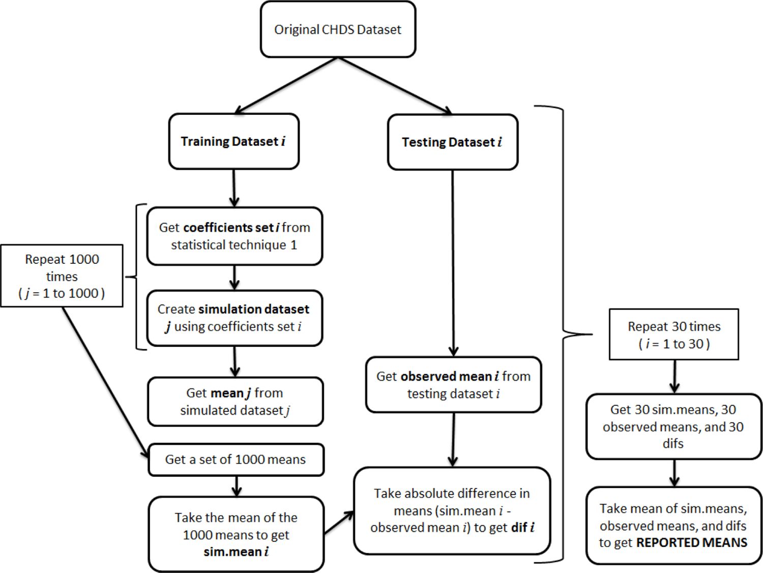
Flowchart showing the cross validation method used to calculate the simulated means, observed means, and the mean absolute differences reported in the results.
The assumptions of each of the models discussed in the review were tested on the entire CHDS dataset (as opposed to using the cross-validation datasets). As most of the tests are performed on the residuals from the model or use the estimated individual effects, usually, separate tests were performed for each model. The details of the tests used for each assumption and the results are provided in Table 3.
R version 3.0.2 was used to programme the simulations and cross-validation process. The OLS-LDV and FE models were estimated using the lm function in R and the AR(1) random effects models were estimated using the glmmPQL R function. SAS 9.3 was used to estimate the variance components random effects and hybrid models. For these models the GLIMMIX procedure was used with the Satterthwaite approximation for the denominator degrees of freedom.
The Stata function xtabond2 was used to fit the two-step system GMM dynamic panel models with orthogonal deviations. The time-variant variables were included as “GMM-style” instruments (as defined by Holtz-Eakin, Newey, and Rosen (1988)). These were collapsed as defined by Roodman (2009b) using the collapse option to reduce the instrument count. The Arellano-Bond test for autocorrelation showed second order autocorrelation in the first differences (equivalent to the within-child errors being serially correlated of order 1) for 29 of the 30 training datasets hence the lags used for instruments were restricted to lag 3 and longer. Third order autocorrelation in the differences was only found for 3 of the 30 training datasets. The final model had 44 instruments to estimate 16 coefficients. The time-invariant variables were treated as exogenous because failure to do resulted in anomalous estimates, possibly due to the proliferation of instruments that are created when specifying GMM-style instruments.
3.1 Assessment measures
The measures calculated in order to compare the six models are described in this section. We first present general definitions of the simulated mean, observed means, and mean absolute differences that are referred to throughout the results. We then provide some further clarification for the specific measures used to assess six different data characteristics. The six data characteristics assessed were: overall distributions, means across time, dynamism, child-specific standard deviations, means by predictor variables, and a general measure of model prediction quality (the prediction sum of squares).
3.1.1 General definition of the plotted simulated means
Let xijka be statistic k, for k in 1 to M, for age a, for a in 9 to 13, on the simulated data for simulation j, for j in 1 to 1000, for cross-validation (CV) dataset i, for i in 1 to 30.
Statistic k could be mean k in a set of three means (M = 3) that are the mean reading scores by the value of a second variable with three levels (e.g., father’s education). Or statistic k could be percentile k in a set of percentiles ranging from 0 to 100 M = 101) calculated for the reading scores or the percentiles for another statistic calculated for each child such as a correlation or standard deviation (e.g. the correlation between reading scores and lagged reading scores for each child and then calculate the percentiles on this set of correlations).
Let xi.ka be the mean over all simulations for statistic k, at age a, for CV dataset i.
Let x..ka be the mean over all simulations and CVs for statistic k, at age a.
The means could be plotted at this stage to compare models at a specific age, but, to enable ease of comparison of models, the summary measures were condensed further by averaging over age to give:
These are the means plotted for the simulated data in Figures 2 to 4.
3.1.2 General definition of the plotted observed means
3.1.3 General definition of the tabled mean absolute differences
Let dika be the difference between observed statistic k and the mean statistic k on the simulated data at age a for CV i.
Let d.ka be the mean of the absolute differences (between observed statistic k and the simulated mean statistic k) over the 30 CVs.
Let d..a be the mean of the absolute values of the d.ka across the full set of statistics (k = 1 to M) (e.g. over the categories of a predictor value or over all 101 percentiles) at age a.
The differences could be examined at specific ages at this stage, but to condense the summary results into a single table the mean was taken over age to give an overall mean absolute difference (between observed and simulated). These are the mean absolute differences presented in Table 4.
3.1.4 Closeness of overall distributions
The overall distribution of reading scores simulated under different statistical models was compared to the distribution of the observed reading scores using percentiles. A cumulative distribution plot was used to show the percentiles from the minimum to the maximum. The values of 101 percentiles from 0 to 100 were calculated. The mean percentiles for the simulated and observed data were calculated as described above in the general definition for simulated and observed means. To quantify the difference between the observed and simulated distributions, the mean absolute difference in percentiles was calculated as described in the general definition above.
3.1.5 Means over time
The mean reading scores at each age were calculated as described in the general definitions above for the simulated and observed means and the absolute differences. Statistic k here refers to a single mean (k in M, where M = 1).
3.1.6 Degree of dynamism (child-specific correlations)
Dynamism exists when there is a relation in a variable from one time-point to the next; the stronger this relationship, the stronger the dynamism. The degree of dynamism in the simulated reading scores under the various statistical techniques was compared to that in the observed reading scores. The measure used to quantify the degree of dynamism was the correlation between the reading scores with the lagged reading scores (the LDV). For a child with reading scores at every age from 8 to 13, five pairs of values are used to calculate this correlation (where a pair is a set of one current and one lagged value). This was calculated individually for each child in the data, providing a vector (length equal to the number of children in the simulation) on which 101 percentiles from 0 to 100 were calculated. The means and differences were calculated as described in the general definitions above with statistic k referring to percentile k (of the distribution of correlations), for k in 1 to M = 101. Plotting these 101 percentiles results in the cumulative distribution plot displayed in Figure 3.
3.1.7 Child-specific standard deviations
For each child, the standard deviation of their reading scores was calculated. Means and differences for plotting and tabling were calculated in the same way as described for ‘Degree of dynamism’ except that rather than using a vector of individual correlations on which percentiles were calculated, a vector of individual standard deviations was used.
3.1.8 Means by other predictors
The mean reading scores by the values of other predictors were calculated as described in the general definitions above for the simulated and observed means and the absolute differences. Statistic k here refers to mean k, for k in 1 to M, where M is equal to the number of levels (categories or unique values for continuous predictors) of the predictor variable.
3.1.9 PRESS statistic
As well as the means and differences described above, we also calculated the prediction sum of squares (PRESS) statistic, a commonly used measure to assess model fit. It measures the closeness of the predicted values of reading score for the test dataset (generated by using the coefficients from the model estimated from a training dataset) to the observed reading scores in the test dataset. Smaller values are better indicating less distance between the predicted and observed values. We used the definition of the standard PRESS as provided in (Mahmood & Khan, 2009). This definition is for a single cross-sectional dataset but as we have 30 CV datasets, which are used for 1000 simulations, and five simulated ages, we calculated this PRESS statistic for each simulation by age by CV combination. We define the PRESS statistic here using notation specific to our situation.
Let yiac be the observed reading score for CV dataset i (i in 1 to 20), at age a (a in 9 to 13), for child c (c in 1 to N) and let be the model predicted reading score (without the addition of any stochastic variation) for simulation j (j in 1 to 1000), for CV i, at age a, for child c. For each CV, for each simulation, for each age, the were subtracted from the yiac to give:
The sum of squares of the djiac was taken over the individual children to give what can be thought of as a simulated sum of squares:
An observed sum of squares was calculated by subtracting the mean observed reading score from each observed reading score, for each CV by age combination and then taking the sum of squares of these differences:
Dividing the simulated sum of squares by the observed sum of squares gives the standard PRESS for a single simulation dataset, i, for a single CV, j, at a specific age, a:
These PRESS statistics were then averaged over simulations, followed by CVs, and finally averaged over age, to give a value for the mean PRESS, PRESS..., which is presented in Table 4.
3.2 An overall summary measure across all data characteristics
The mean absolute differences (MADs) reported in Table 4 can illuminate which models were performing the best for different data characteristics but, additionally, an overall summary measure was created to compare models across all data characteristics. The means presented in Table 4 were standardised across each row (for each data characteristic) by taking the values in that row, subtracting the mean and then dividing by the standard deviation of these values. This created standardised mean absolute differences (SMADs) where more negative values indicated simulated data that was closer to the real data. By standardising across rows, the means became comparable down columns and an overall summary measure could be created by taking the mean down the column for each model. The summary mean allows an overall comparison between the techniques of the closeness of the simulated data to the real data across all the data characteristics assessed.
Weighted means were computed because too much weight would be given to the ‘means by predictors’ data characteristics if a raw mean were computed. We employed two weighting schemes. In the first we treated the ‘means by time-invariant predictors’ and ‘means by time-variant predictors’ characteristics as a single data characteristic when taking an overall average summary measure. Using a weight of 1/5 for each of the five ‘means by time-invariant predictors’, a weight of 1/3 for each of the three ‘means by time-variant predictors’, and a weight of 1 for all other data characteristics accomplished this purpose. In the second weighting scheme the eight ‘means by predictors’ characteristics were considered a single data characteristic To accomplish this, the weights for the five measures for time-invariant predictors should sum to 0.5 (giving each a weight of 0.5/5 = 0.1) and the weights for the three measures for time-variant predictors should sum to 0.5 (giving each a weight of 0.5/3 = 1/6). The weights for the other data characteristics remained at 1.
The mean absolute differences were also examined for each age separately; tables equivalent to Table 4 were created for each age (available in the online Appendix). The overall weighted mean summary measures for each model were computed at each age and those using the first weighting scheme are shown in Table 5.
3.3 Significance Testing
Comparing the simulated and observed means (by examining graphs) and the mean absolute differences provides a descriptive comparison but does not tell us if one model is significantly better than another. Significance testing for each data characteristic was performed for this purpose.
Paired t-tests, paired by CV, were used to test whether pairs of models differed significantly for a specific statistic (e.g. a specific percentile, a specific category or value of a predictor). The values used for the tests were the 30 absolute differences (between simulated and observed values) averaged over the 1000 simulations, averaged over age (the dika averaged across a, giving 30 values for a specific k) for any two models being compared. The values were averaged across age so that the t-tests corresponded to the mean absolute differences presented in Table 4. A comparison of values from different models found that values from the same CV were found to be more similar to each other than values from different CVs (inspected by scatterplots) for many of the data characteristics and hence paired t-tests were used through-out.
Assumptions made for each model. ✓A indicates that the assumption is made by the model. Following this may be either the result of testing for the assumption or a comment (A dash (-) indicates that the test is not relevant).
| Assumption | Test used | OLS-LDV | RE | RE-AR(1) | FE | HYBRID | GMM Dynamic Panel | |
|---|---|---|---|---|---|---|---|---|
| 1 | No individual effects: μi = 0, εi,t = υi,t | LR test for non-zero , p-value based on a mixture of chi-squares (COVTEST in the GLIMMIX procedure, SAS 9.3). | ✓ A, LDV in model: x2(1) = 0.00, p = .9999; LDV not in model: x2(1) = 7958, p < .0001 | - | - | - | - | - |
| 2 | Individual effects independent of within-child errors: Cov(μi, υi,t = 0 | Test for Pearson’s correlation between estimated individual effectsa and residuals | - | ✓A, , p < .0001 | ✓A, , p < .0001 | |||
| 3 | Individual effects independent of each other: μi~iid | Assumed by virtue of the individuals being randomly selected and from different families | - | ✓A | ✓A | μis eliminated by transformation | ✓A | μis eliminated by transformation |
| 4 | μi~N(0.σb) | Shapiro-Wilk test on the empirical BLUPsb of individual effects | - | ✓A, W = 0.99, p = .0001, but plotting shows distribution close to normal | ✓A, W = 0.99, p < .0001, but plotting shows distribution close to normal | ✓A, W = 0.99, p = .0001, but plotting shows distribution close to normal | ||
| 5 | Cross-sectional ‘between’ effects equal to within ‘fixed’ ,, . K = λ effects: k = λ | Hausman test | ✓A, x2(5) = 2.55, p = .7693 | ✓A, x2(5) = 2.55, p = .7693 | ✓A, x2(5) = 2.55, p = .7693 | Only λ estimated | λ and κ estimated separately | Only λ estimated |
| 6 | Exogenous time-invariant predictors (TIPs): Cov(υi,t, xi,t) = 0, Cov(zi, υi,t) = 0, | C statistic from endogtest in stata’s ivreg2c | ✓A, null of exogeneity not rejected for any TIPsd. LDV endogenous by definition. | ✓A, null of exogeneity rejected for most TIPse | ✓A, no convenient test – refer to tests for RE model | TIPs not used | ✓A, null of exogeneity rejected for half of the TIPse | Diff GMM: TIPs not used. System GMM: Assumption does not need to be made |
| 7 | Exogenous time-variant predictors (TVPs): Cov(εi,t, xi,t) = 0, Cov(μi, ) = 0 | C statistic from endogtest in stata’s ivreg2 or xtivreg2c | ✓A, null of exogeneity rejected for one TVPd | ✓A, null of exogeneity rejected for two TVPse | ✓A, no convenient test – refer to tests for RE model | ✓A, null of exogeneity not rejected for any TVPsf | ✓A, null of exogeneity rejected for one TVPe | Assumption does not need to be madeg |
| 8 | υi,t~iid N(0, σ2): Within-child errors serially uncorrelated | System GMM: Arellano-Bond test for AR in first differences Other models: xtserial in stata (Wooldridge 2002) | ✓A, F(1, 1003) = 398.5, p < .0001 | ✓A, F(1, 1043) = 115.5, p < .0001 | Assumes an AR(1) structureh | ✓A, F(1, 1043) = 115.5, p < .0001 | ✓A, F(1, 1043) = 115.5, p < .0001 | Assumption not made but choice of instruments depends on degree of serial correlation. instruments depends on degree of serial correlation. AR(2): z = 4.33, p < .0001. AR(3): z = -1.60, p = .109. |
| 9 | υi,t~iid N(0, σ2) Within-child errors independent across individuals (no cross-sectional dependence) | Pesaran’s test (Pesaran 2004): xtcsd in stata | - | ✓A, statistic = 6.62, p < .0001 | ✓A, no convenient test – refer to test for RE model | ✓A, statistic = 6.45, p < .0001 | ✓A, no convenient test – refer to tests for RE and FE models | ✓A, no convenient test – refer to tests for RE and FE models |
| 10 | Validity of moment conditions (validity of instruments) for Difference GMM | Hansen test | - | - | - | - | - | ✓A, x2(22) = 24.47, p = .323 |
| 11 | Validity of additional moment conditions for System GMM | Difference in Hansen test | - | - | - | - | - | ✓A, x2(4)=16.27, p=.003 |
| 12 | Stationarity of within-child errors | Hadri and Larsson (2005) | Z = -2.80, p = .0051 | Z = 19.31, p < .0001 | Z = 19.46, p < .0001 | Z = 19.34, p < .0001 | Z = 19.32, p < .0001 | System GMM: Z = -2.80, p = .0051 |
-
a
Estimated individual effects were the empirical BLUPs (best linear unbiased predictors) estimated by SAS
-
b
BLUP = best linear unbiased predictor. Empirical BLUPs estimated in SAS by requesting fitted values with and without BLUPS and taking the difference.
-
c
The tests utilised additional variables not included in any models as excluded instruments (each tested for exogeneity and relevance). Predictors were tested individually with all other variables in the model treated as exogenous. Each model was checked for identification and weak. Significance was set at the .05 level. Full results of the tests and stata code are available in the online Appendix.
-
d
LDV included in the model. cluster option not used (panel data structure ignored).
-
e
LDV not included in the model. cluster option used to indicate panel data structure.
-
f
LDV not included in the model. cluster option used to indicate panel data structure. fe option used.
-
g
Although the exogeneity if variables should be investigated so that the analyst has some indication of what variables need to be instrumented and which do not.
-
h
A test for whether the AR(1) structure was defensible compared to an unstructured structure was attempted in SAS but the model with the unstructured model would not converge
The t-values from the tests are reported in tables in the online Appendix. The t-values were not adjusted for multiple testing but left to be interpreted based on their relative size or a specific level of significance can be assessed by obtaining the relevant critical value. For interpretation in the results section, we considered models to be significantly different if the t-value was greater than 2.46 (a .01 level of significance with the 29 degrees of freedom associated with the tests).
4. Results
4.1 Testing Model Assumptions
Table 3 shows the results of testing the various assumptions made by each of the models on entire CHDS dataset. For all tests, a small p-value provides evidence of a violated assumption. Evidence of violated assumptions was present for all of the models and choosing a model that is theoretically best based on the assumptions testing is not clear. Some assumptions may be more important than others but testing the effect of breaking each individual assumption is beyond the scope of this article.
The OLS-LDV model assumes no individual effects and so the assumptions regarding individual effects do not apply. This may make it appear that the number of violated assumptions is small compared to other models; however the violation of this key assumption, along with the fact that the inclusion of the LDV creates bias by definition, indicates that perhaps one of the other models should be preferred, even if they also have assumptions that are violated. The empirical assessment aims to test which models perform the best on our specific dataset, even though, for each, there is evidence of violated assumptions. Although the system GMM dynamic panel model does not make many of the assumptions the other models make, the violation of the assumption regarding the additional moment conditions (necessary to estimate effects for time-invariant variables) could be very important; again, the empirical assessment aims to give some light as to how important.
Mean absolute differences (MAD) (smaller is better) and standardised mean absolute differences (SMAD) (more negative is better) between simulated and observed data.
| Data characteristic | OLS – LDV | RE) | RE-AR(1) | FE | HYBRID | SYSTEM GMM | |||||||
|---|---|---|---|---|---|---|---|---|---|---|---|---|---|
| MAD | SMAD | MAD | SMAD | MAD | SMAD | MAD | SMAD | MAD | SMAD | MAD | SMAD | ||
| PRESS statistica | 0.53 | −0.11 | 0.44 | −0.66 | 0.81 | 1.59 | 0.39 | −0.99 | 0.44 | −0.64 | 0.68 | 0.80 | |
| Overall distributions | 1.47 | −0.97 | 2.66 | 0.07 | 4.70 | 1.86 | 2.08 | −0.44 | 2.69 | 0.10 | 1.87 | −0.62 | |
| Means across time | 0.50 | −1.42 | 0.69 | −0.05 | 0.70 | −0.01 | 0.73 | 0.23 | 0.93 | 1.66 | 0.64 | −0.41 | |
| Child-specific correlations (dynamism) | 0.09 | −1.45 | 0.23 | 0.85 | 0.24 | 0.92 | 0.15 | −0.46 | 0.23 | 0.82 | 0.14 | −0.68 | |
| Child-specific standard deviations | 0.76 | −1.75 | 1.07 | −0.27 | 1.38 | 1.19 | 1.16 | 0.14 | 1.13 | 0.02 | 1.27 | 0.66 | |
| Time invariant predictors: | |||||||||||||
| Gender | 0.72 | −1.51 | 1.16 | 0.19 | 1.15 | 0.15 | 1.38 | 1.02 | 1.37 | 0.98 | 0.90 | −0.82 | |
| Breast-feeding | 1.69 | −0.77 | 1.82 | −0.42 | 2.74 | 1.97 | 1.77 | −0.57 | 1.97 | −0.04 | 1.92 | −0.17 | |
| Father’s education | 0.85 | −1.64 | 1.19 | −0.15 | 1.51 | 1.18 | 1.38 | 0.64 | 1.34 | 0.47 | 1.11 | −0.51 | |
| Mother’s education | 0.91 | −1.46 | 1.29 | −0.04 | 1.68 | 1.43 | 1.35 | 0.19 | 1.45 | 0.56 | 1.12 | −0.67 | |
| Family’s socio-economic status | 0.94 | −1.49 | 1.06 | −0.72 | 1.38 | 1.36 | 1.21 | 0.28 | 1.25 | 0.56 | 1.17 | 0.01 | |
| Time-variant predictors: | |||||||||||||
| Home-ownership | 1.07 | −0.64 | 1.29 | −0.45 | 1.60 | −0.18 | 1.20 | −0.53 | 1.57 | −0.21 | 4.19 | 2.01 | |
| Mother’s hours worked | 4.81 | −0.61 | 4.95 | −0.49 | 7.88 | 1.86 | 4.63 | −0.75 | 5.01 | −0.44 | 6.10 | 0.43 | |
| Father’s smoking | 5.31 | −0.80 | 5.73 | −0.51 | 8.42 | 1.36 | 5.34 | −0.78 | 5.80 | −0.46 | 8.17 | 1.19 | |
| Weighted means | |||||||||||||
| Scheme 1b | −1.11 | −0.11 | 1.11 | −0.27 | 0.30 | 0.08 | |||||||
| Scheme 2c | −1.12 | −0.07 | 1.11 | −0.28 | 0.34 | 0.02 | |||||||
-
a
The PRESS statistic is not a mean absolute difference but a standardised measure of the distance between the observed and predicted values. Smaller values are better.
-
b
Time-invariant predictors given a weight of 1/5 each, time-variant predictors given a weight of 1/3 each. Other characteristics each given a weight of 1.
-
c
Means by predictor variables given a combined weight of 1 with the time-invariant predictors each given a weight of 0.1 and the time-variant predictors each given a weight of 1/6. Other characteristics each given a weight of 1.
4.2 Comparison of means between models
Figures 2 to 4 display the means, for each of the assessment measures described above, from data simulated using the coefficients from each of the models, alongside the observed means. Table 4 shows a summary of the mean absolute differences between the simulated and observed means. These values were based on taking the mean, over the cross-validations, of the absolute differences between simulated and observed statistics. In contrast, for the means plotted in the graphs, the overall mean of the simulated statistics are shown; means of absolute differences were not taken. A comparison of the simulated and observed means in the graphs is an examination of bias. The simulated means show the average difference, over the cross validations, rather than the average absolute difference. Points or lines that look close to the observed values on the graphs could have a large variance across cross-validations. The mean absolute differences in Table 4 are similar in concept to the mean squared error – they incorporate the aspects of bias (accuracy – how close we get to the observed values on average) and variance across cross-validations (precision). The means in the graphs only inform about bias.
The comparison of the means in the graphs and the mean absolute differences in Table 4 provides a descriptive comparison between the models and allows a ranking across them; however, it does not tell us if one model is significantly better than another. Significance testing for each data characteristic was performed for this purpose. A brief summary of the results is included in this section and the full set of results is provided in the online Appendix. A .01 level of significance was used.
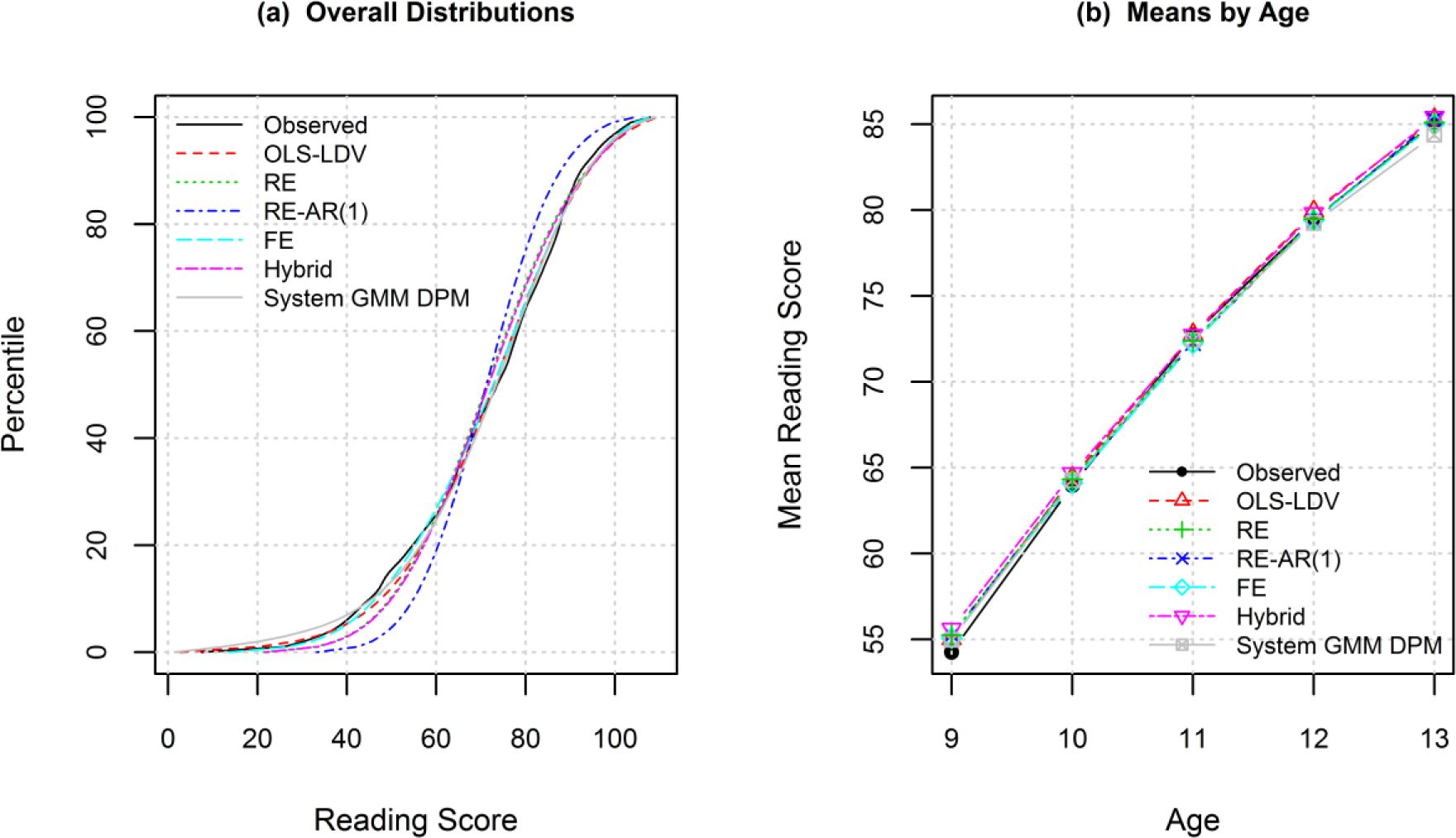
Figure 2a shows the cumulative distributions for the observed reading scores and the reading scores simulated under the different statistical models. All models reproduced the distribution reasonably well. The values in Table 4 reveal that the reading scores simulated using the OLS-LDV model were closest to the observed distribution, followed by the system GMM dynamic panel model (not significantly different from OLS-LDV), and then the fixed effects model. The OLS-LDV model was significantly better than the RE and hybrid models and the system GMM model was significantly better than the hybrid model. The random effects AR(1) model performed the worst (significantly worse than all other models).
The mean reading scores by age are shown in Figure 2b for the observed data and the data simulated under the different statistical modelling methods. All the models appear to perform well. The means calculated from the OLS-LDV model were the closest to the observed means, followed by the system GMM model (see Table 4) (models only significantly different at age 13). The OLS-LDV model performed significantly better than the hybrid model at all ages.

Comparison of the observed reading scores and the reading scores simulated under the six models.
(a) Cumulative distribution curves for the overall distributions.
(b) Means by age.
Figure 3a shows cumulative distributions of the child-specific correlations. All of the models underestimated the degree of dynamism. The correlations from the OLS-LDV model were closest to the observed distribution, followed by those from the system GMM model (see Table 4). The differences between these models were significant at all percentiles tested. The system GMM model performed significantly better than the hybrid, RE, and RE-AR(1) models.
Figure 3b shows cumulative distributions of the child-specific standard deviations. All the models perform reasonably well, but the standard deviations calculated under the OLS-LDV model tracked the closest to the observed distribution. The distributions for the standard RE and hybrid models were extremely similar. Table 4 revealed that the standard RE model performed second best, followed by the hybrid model. Fourth was the FE model which also had a very similar shape to the RE and hybrid models. Significance results varied across percentiles and no simple conclusions could be made.

Cumulative distribution curves of the observed reading scores and the reading scores simulated under the six models.
(a) Child-specific correlations of current and lagged score
(b) Child-specific standard deviations.
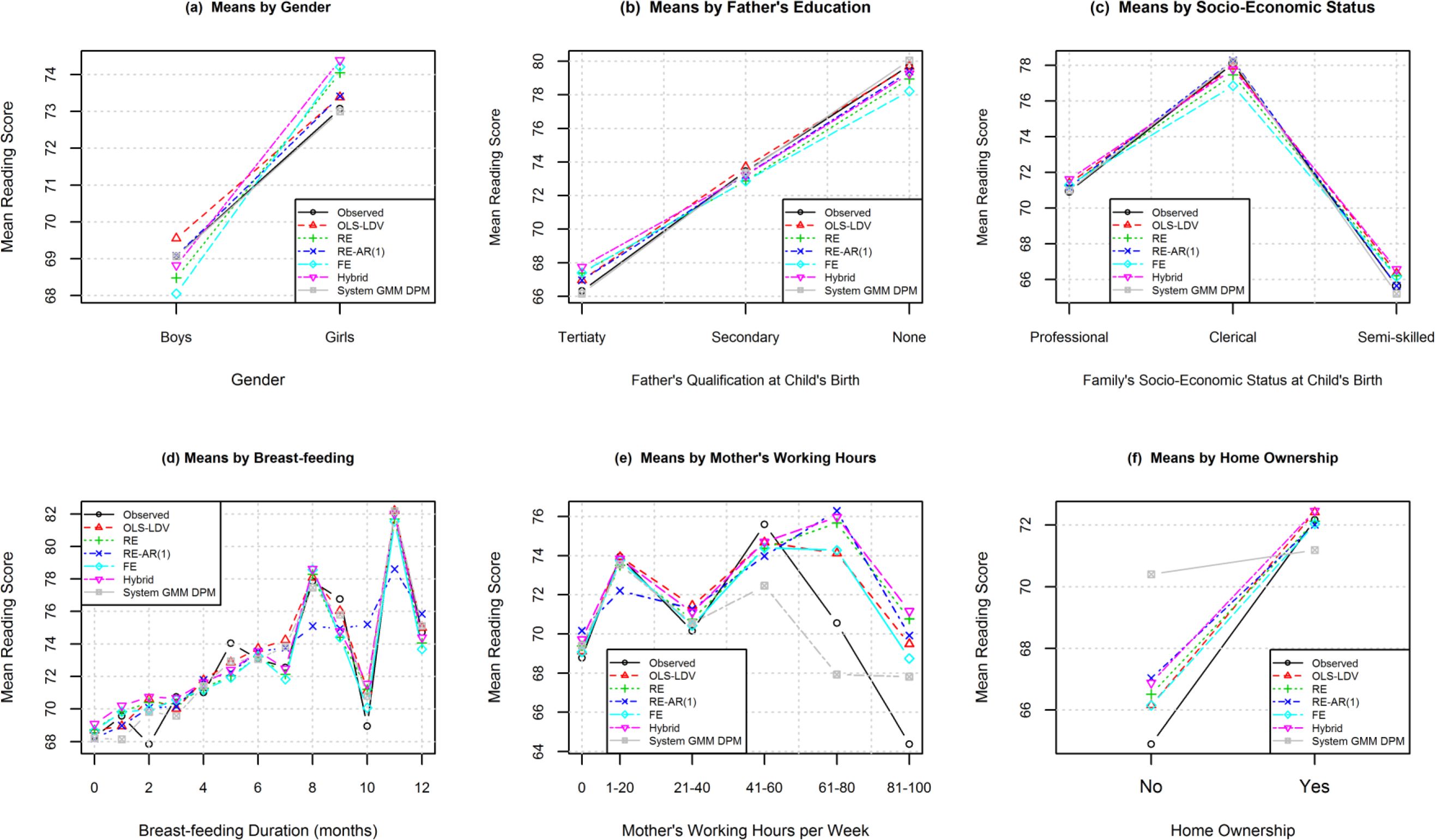
Figure 4 shows the mean reading scores by the values of a predictor variable for six of the eight predictors in the models. Recall that the values in the graph inform only about bias. For gender (4a), the graph shows the means from the system GMM model being the closest to the observed means, with those from the RE-AR(1) and OLS-LDV model looking next best. However Table 4 ranks the OLS-LDV model as the best performer with system GMM ranked second. The system GMM technique produces means that have a larger variance across the cross-validations such that the absolute values of the differences (means in Table 4) from the observed means are smaller for the OLS-LDV model. The OLS-LDV model was significantly better than the system GMM models for the mean for girls only. The OLS-LDV model performed significantly better than the RE, RE-AR(1), hybrid, and FE models. The FE model ranked last performing significantly worse than system GMM and RE.

Comparison of observed and simulated mean reading scores by predictors.
(a) By gender. (b) By father's education. (c) By socio-economic status. (d) By breast-feeding. (e) By mother's working hours. (f) By home-ownership. Lines joining points are added to make distinctions between models more clear.
For father’s education (4b) (a time-invariant predictor), the situation is similar to that for gender: from the graph, the system GMM model looks the best but Table 4 revealed that the OLS-LDV model performed the best in terms of absolute differences indicating greater variability in means across CVs for the GMM models. Table 4 ranked the system GMM model second; it was significantly worse than the OLS-LDV model at the tertiary and secondary levels of education. The OLS-LDV model was significantly better than the RE-AR(1) hybrid model at all categories.
The results for mother’s education (plot not shown) showed a similar pattern to that seen for father’s education except with the order of hybrid and FE models switched. The only comparison that was significant at all categories was that between the OLS-LDV model and the RE-AR(1) model, which ranked last.
For socio-economic status (SES) (4c), all models matched the observed pattern of means reasonably well. Table 4 shows the OLS-LDV model ranking the best, followed by the standard RE model. The significance results varied by SES category, with the only comparisons consistent across all categories being the non-significance between system GMM and RE, hybrid, and FE and between REAR1 and hybrid.
For breast-feeding (4d), all the models appear to follow a similar pattern to each other except for the means from the RE-AR(1) model which follow a smoother line. Table 4 revealed RE-AR(1) as the worst performer and OLS-LDV as the best performer, followed by FE. OLS-LDV was significantly better than RE-AR(1) at all durations of breast-feeding tested.
In order to present a clear plot, mother’s working hours (4e), was categorised and the mean reading scores calculated for each category. From the graph we judge that means from the OLS-LDV and FE models are closest to the observed. This is also found in Table 4 with FE ranking first and OLS-LDV ranking second. The only clear pattern from the significance testing was that the RE-AR(1) model (ranked last) performed significantly worse than the FE and RE models.
For home-ownership (4f), system GMM was clearly the worst performer, being significantly worse than all other models for the ‘not owned’ category. In Table 6, which shows the coefficients for each of the models, we see that the coefficient for home-ownership is quite different to that for the other models, resulting in the difference observed in the figure. From the graph we see that the OLS-LDV and FE models appear to be the best. Table 4 ranked OLS-LDV the best and then FE. The OLS-LDV model performed significantly better than all models for the ‘owned’ category. For the ‘not owned’ category, most of the models differed significantly from each other, except for OLS-LDV with RE, hybrid and FE and for RE-AR(1) with hybrid.
For father’s smoking (plot not shown), the ranks in Table 4 are similar to those for the other time-variant predictors with OLS-LDV ranking first and FE ranking second. The OLS-LDV model was significantly better than all other models for the tests conducted at zero and four cigarettes smoked per day except for system GMM at four cigarettes per day.
To give an overall ranking of the models across all the data characteristics assessed, a weighted mean of the standardised mean differences was calculated for each model (last two rows in Table 4). By this criterion, the OLS-LDV model performed the best on average, followed by the FE model. The standard RE model came third, the system GMM dynamic panel model came fourth, the hybrid model came fifth, and the RE-AR(1) model ranked last. The results were also examined separately for each age (tables by age available in the online Appendix) and the overall summary measure weighted according to scheme 1 is shown for each age in Table 5. Although there are trends over time within models, the pattern of the means across models at a given age is the same and the overall conclusions that would be made from examining the results separately for each age are the same as what are made when averaging across age.
Overall weighted mean of the standardised mean absolute differences (using weighting scheme 1a) by age for each model.
| AGE | MEAN OVER AGEb | |||||
|---|---|---|---|---|---|---|
| MODEL | 9 | 10 | 11 | 12 | 13 | |
| OLS – LDV | −1.11 | −1.10 | −1.10 | −1.06 | −1.04 | −1.11 |
| RE | −0.08 | −0.07 | −0.06 | −0.11 | −0.11 | −0.11 |
| RE-AR (1) | 1.22 | 1.18 | 1.09 | 0.94 | 0.74 | 1.11 |
| FE | −0.16 | −0.24 | −0.27 | −0.30 | −0.27 | −0.27 |
| Hybrid | 0.42 | 0.34 | 0.28 | 0.28 | 0.24 | 0.30 |
| System GMM | −0.29 | −0.09 | 0.05 | 0.25 | 0.44 | 0.08 |
-
a
Time-invariant predictors given a weight of 1/5 each, time-variant predictors given a weight of 1/3 each. Other characteristics each given a weight of 1.
-
b
The weighted mean of the SMADs that were averaged over age. This is the same value as shown in the second-to-last row of Table 4.
Coefficients and standard errors estimated on the full dataset for each of the techniques.
| Variable | OLS – LDV | RE | RE-AR(1) | FE | Hybrid | System GMM DPM 2 Step a | System GMM DPM 1 Step a | |
|---|---|---|---|---|---|---|---|---|
| Reading score previous centred (LDV) | 0.90 | 0.83 | 0.82 | |||||
| (0.01) | (0.04) | (0.04) | ||||||
| Reading score previous centred squared (LDV squared) | −0.00 | −0.01 | −0.01 | |||||
| (0.00) | (0.00) | (0.00) | ||||||
| Child’s age centred | −0.33 | 8.02 | 7.98 | 8.01 | 8.02 | 0.23 | 0.27 | |
| (0.09) | (0.05) | (0.10) | (0.05) | (0.05) | (0.41) | (0.41) | ||
| Child’s age centred squared | 0.13 | −0.52 | −0.06 | −0.51 | −0.52 | −0.01 | −0.02 | |
| (0.04) | (0.03) | (0.03) | (0.03) | (0.03) | (0.10) | (0.10) | ||
| Gender (reference: Female) | 0.07 | −3.78 | −3.31 | −3.79 | 0.51 | 0.49 | ||
| (0.21) | (0.98) | (0.75) | (0.98) | (0.34) | (0.35) | |||
| Father’s education (reference: No formal education) | Tertiary | 1.43 | 6.78 | 5.10 | 6.54 | 0.68 | 0.51 | |
| (0.39) | (1.79) | (1.37) | (1.81) | (0.58) | (0.57) | |||
| Secondary | 0.98 | 4.60 | 3.57 | 4.56 | 0.67 | 0.71 | ||
| (0.25) | (1.18) | (0.90) | (1.18) | (0.36) | (0.36) | |||
| Mother’s education (reference: No formal education) | Tertiary | 1.01 | 7.02 | 5.16 | 6.76 | 1.18 | 1.05 | |
| (0.32) | (1.53) | (1.17) | (1.55) | (0.55) | (0.54) | |||
| Secondary | 0.42 | 2.47 | 1.65 | 2.31 | 0.47 | 0.40 | ||
| (0.26) | (1.21) | (0.92) | (1.21) | (0.37) | (0.35) | |||
| Family’s socio-economic status (reference: Semi-skilled) | Professional | 0.22 | 4.28 | 3.37 | 3.76 | 0.71 | 0.22 | |
| (0.39) | (1.79) | (1.37) | (1.82) | (0.72) | (0.77) | |||
| Clerical | 0.03 | 2.43 | 1.97 | 2.02 | 0.18 | −0.14 | ||
| (0.27) | (1.23) | (0.93) | (1.25) | (0.54) | (0.56) | |||
| Breast-feeding | 0.07 | 0.26 | 0.20 | 0.25 | 0.05 | 0.06 | ||
| (0.03) | (0.13) | (0.10) | (0.13) | (0.03) | (0.03) | |||
| 0.00 | 0.01 | 0.00 | 0.01 | (D, M): 0.01, 0.01 | −0.02 | 0.01 | ||
| Mother’s hours worked | (0.01) | (0.01) | (0.01) | (0.01) | (0.01), (0.04) | (0.04) | (0.04) | |
| Father’s smoking | 0.00 | −0.03 | −0.01 | −0.03 | (D, M): -0.02, -0.09 | −0.16 | −0.24 | |
| (0.01) | (0.02) | (0.02) | (0.02) | (0.02), (0.07) | (0.12) | (0.11) | ||
| Home-ownership (reference: owned/mortgaged) | −0.72 | −1.48 | −1.15 | −1.30 | (D, M): -1.31, -3.75 | 3.66 | 2.29 | |
| (0.30) | (0.43) | (0.42) | (0.44) | (0.45), (1.62) | (2.98) | (3.18) | ||
-
D: For the hybrid technique, estimate of the within / fixed effect calculated from the deviation variable.
-
M: For the hybrid technique, estimate of the between/cross-sectional effect calculated from the mean variable.
-
a
Windmeijer corrected standard errors are displayed
4.3 Model coefficients
Table 6 shows the coefficients estimated from each technique using the entire CHDS dataset. For interest, the coefficients estimated from a one-step system GMM model are also shown, although this model was not included in the empirical assessment as the coefficients were very similar.
5. Discussion
Micro-simulation models are being increasingly used, particularly in areas with policy application (Spielauer, 2010). To date however, there has been little discussion on the different models options for estimating the parameters that drive the MSM and how to choose between them. Technical reports for DMSMs (found in the ‘grey’ literature) sometimes provide comments on different techniques considered by the group, but examples of systematic comparisons are lacking.
Hence, the aim of this paper, published in a peer-review journal, was to demonstrate some ways of comparing regression-style modelling techniques in terms of how they perform at generating simulated data when their parameter estimates are applied to a discrete-time DMSM. This can be thought of as a kind of validation of a DMSM. Most reported validation for microsimulation focuses on aggregate means over time or by some key groups. The longitudinal unit-specific aspects of validation (such as dynamism and child-specific standard deviations) are not often examined as undertaken here.
The statistical techniques assessed were an ordinary least squares regression with a lagged dependent variable (OLS-LDV), two random effects techniques: one with a variance components within-child error structure and one with an autoregressive order 1(AR(1)) within-child error structure, a hybrid model, and a dynamic panel model (DPM) estimated with system general method of moments (GMM). We simulated reading scores under the coefficients and assumptions of each model and assessed how well each simulated set of reading scores compared to the observed reading scores from our birth cohort data. The assessment does not provide general results on which modelling techniques are best for generating artificial data but provides an illustration of how one might go about comparing and testing different model specifications.
In addition to illustrating how simulated data from different models can be compared, a review of the assumptions of these commonly used modelling techniques has been provided. In our data assumptions were violated for all the models and hence the empirical assessment also provided an indication of the importance of meeting these assumptions for our MSM. We found that it was still possible to generate synthetic data that represent reality when the assumptions of a statistical model are violated.
Although the OLS-LDV technique had the strictest set of assumptions, it had a number of advantages. It was simple to execute in statistical software and to implement in the simulation and performed the best overall in our assessment comparing the simulated to observed reading scores.
The fixed effects technique ranked second in the empirical assessment; however it was not considered a feasible modelling option for out MSM because scenarios on time-variant variables would not be able to be performed. We found only two DMSMs that used fixed effects models: a DMSM for the income of the Dutch elderly (Knoef, Alessie, & Kalwij, 2013) and the MINT model (Toder et al., 2002). In the first version of MINT, the fixed effects technique was used to predict earnings; however, they found that their predictions were not ideal, so in MINT3 the fixed effects technique was replaced by a hot-deck imputation approach (Toder et al., 2002:II-2–3). However, they did choose to use the fixed effects technique in MINT3 for pre-retirement earnings after age 50.
The random effects technique, ranking third overall, also performed reasonably well on all aspects, except perhaps on dynamism where it ranked second-to-last. The system GMM dynamic panel model came out fourth overall. This technique ranked high on some data characteristics and low on others. It did not perform well in replicating means by time-variant predictors; this is likely due to weak instrumentation and violation of assumptions on the instruments. The system GMM model also ranked poorly for replicating the child-specific standard deviations. It performed well in terms of replicating the overall distribution, means across time, and the child-specific correlations.
Dynamic panel GMM estimators are complicated; there are many choices that need to be made and given their complexity it is relatively easy for non-experts to violate assumptions and generate invalid estimates. We experimented with different options for the GMM model and did not find any specifications that resulted in sensible looking estimates (except for one-step estimation instead of two-step for the model used in the empirical assessment, which gave similar estimates, as reported in Table 6); however, it is possible that further perseverance with GMM model specifications could result in simulated data that performs better than that reported here.
As far as we are aware, no DMSM has used a GMM dynamic panel model technique. Emmerson, Reed, and Shephard (2004), in their review of PenSim2, suggested that, to account for the endogeneity of the LDV, the dynamic panel model GMM estimator be used as an alternative to their random effects approach in modelling earnings (p. 33). This would be a good approach to investigate, although our work suggests that a dynamic panel GMM estimator will not necessarily perform better.
Although the hybrid technique had some theoretical advantages over the random effects model, it ranked fifth overall. Even so, the simulated means and distributions were not wildly different from those from the other models. The significance testing, however, found that the hybrid model performed significantly worse that the OLS-LDV model for overall distributions, means over time, dynamism, and mean reading scores by gender and father’s education. We did not find any cases of DMSMs using a hybrid model, most likely due to the hybrid technique being less commonly known.
The random effects model with AR(1) within-child errors ranked last. Given that this model performed worse than the standard random effects model (with a variance components error structure), this indicates the AR(1) structure was not a good fit to our data. Further within-child error structures could be investigated and some improvement on the standard RE model could be gained. For use in a DMSM however, one would also have to consider how other within-child error structures could be implemented in the simulation of data.
If creating a DMSM, the use of the random effects, hybrid, or fixed effects models lead to further decisions that must be made regarding the individual effects. There are multiple options for assigning individual effects at the start of the simulation which need to be considered (although Richiardi’s Rank Method ((Richiardi, 2014) and (Richiardi & Poggi, 2014)) is a compelling choice given the lack of bias and ease of implementation) and there is also the question of how to treat the individual effects during the running of scenarios: are they left as per the status quo base simulation or are there scenario options that can change the distribution of individual effects for the population or a subgroup of the population?
It was interesting that the rank order of the PRESS statistic did not follow a pattern similar to the ranks for the other data characteristics assessed. For microsimulation it is important that we generate data that is similar in multiple ways to the real world; in addition to generating the overall distribution of a variable, we also want to maintain associations between variables and longitudinal relationships over time (dynamism). The PRESS statistic measures the closeness of the fitted values to the observed values but does not measure these other characteristics and so, although the most well-known of our assessment measures, it was not the most important one in our opinion.
Significance testing was performed for each data characteristic at specific values (e.g. specific levels of predictor variables or specific percentiles), giving a large number of tests. It was difficult to summarise the patterns observed; just over half of the tests gave evidence of a difference between models. The most commonly observed pattern was that the best performing model (the OLS-LDV model except for means by mother’s working hours) was usually significantly better than the models ranked last or close to last. This indicated to us that choosing any of the highly ranked models would be reasonable based on the significance tests.
The choice of model for parameter estimation may depend on what aspects of the data are important to reproduce. If our microsimulation were not dynamic, the random effects model may be more seriously considered as simulating dynamism (e.g. by including an LDV in the model) would not be an issue. The decisions on which model to choose can be made based on multiple criteria. For microsimulation these could be the performance of potential models in an empirical assessment as undertaken here, any reservations over violated model assumptions, the ease of implementation in the simulation, and any further issues relating to scenario testing. For our dynamic MSM, the OLS-LDV technique appeared to be a defensible choice. Indeed we found this to be the most commonly used regression method for simulating a continuous state-dependent variable (see Table 1).
For applications other than microsimulation, the criteria for making decisions could be different. For example, if one was interested in the effect of one key time-variant predictor on an outcome and only wanted to control for other variables (i.e., was not interested in the effect of them on the outcome) then fixed effects or difference GMM may be best. However, the principles discussed here on considering model assumptions and experimenting with different model specifications would still hold.
We performed no variable selection in our empirical performance assessment but fit each model with the same set of pre-determined variables. This eliminated variation and potential bias from the variable selection process. In practice, however, variable selection may be performed, so it would be interesting to repeat this empirical assessment performing variable selection for each method.
We assessed six models in our empirical work, but of course there are many other statistical modelling techniques that could be included in an assessment like this. In addition to other regression-style techniques for parameter estimation, there are methods that require more specialised programming that estimate parameters by minimising an objective or distance function.
Simulated minimum distance is one such approach that has been suggested for agent-based models (Grazzini & Richiardi, 2015) and could be considered for microsimulation also.
The discussion of the six chosen modelling techniques is also useful to analysts choosing statistical techniques for other purposes (e.g. fitting a model to test associations). We explained how one would execute these techniques in statistical software and the table of assumptions lays out essential knowledge in choosing an appropriate modelling technique: it shows, at a glance, what assumptions a model makes and a test to evaluate the likelihood of the assumption being met.
6. Conclusion
Modellers have options when it comes to choosing modelling techniques; they should make their choice carefully, considering the assumptions of the techniques, the importance of simulating different aspects of the data, the implementation of estimated parameters in the MSM, and the ultimate application and aims of the MSM. Our assessment here aims to encourage modellers to experiment with different models in the process of making this choice. We demonstrated various criteria that can be used to assess the performance of parameter estimates from a model in reproducing observed data. For our specific data we found that data simulated from parameters from an OLS regression model with an LDV most closely represented the observed data. The fixed effects model performed second best followed by the standard random effects technique, and then the system GMM dynamic panel model and the hybrid model. The random effects AR(1) model ranked last. For the most part, however, all of the models generated synthetic data that replicated the observed data to a reasonable degree, with certain models performing better or worse on particular data characteristics. Although the simplest technique of an OLS regression including an LDV was found to perform well in our case, this result cannot be considered generalizable. Given the potential bias in the estimates from this model due to the violation of assumptions, it will be important for other modellers to perform their own sensitivity analysis to gain insight into the confidence they can have in using this technique (or any others where assumptions are broken) for their MSM or research application. We hope the comparative assessment performed here will result in more modellers comparing the effects of different modelling choices, which will ultimately help to improve the quality of, and strengthen the confidence in, microsimulation models and other research based on statistical models.
1. Mean absolute differences and standardised mean absolute differences data at each age
Tables 1 to 5 show the Mean absolute differences (MADs) and standardised mean absolute differences (SMADs) between simulated and observed data for each age. These values are equivalent to those presented in Table 4 in the main text except that they use data only from one of the ages (e.g. only the age 8 data in used in Table #) and no averaging across age has occurred as was performed for the values in Table 4 in the main text.
Mean absolute differences (MAD) (smaller is better) and standardised mean absolute differences (SMAD) (more negative is better) between simulated and observed data for age 9.
| OLS-LDV | RE | RE-AR (1) | Hybrid | FE | System GMM DPM | |||||||
|---|---|---|---|---|---|---|---|---|---|---|---|---|
| Data Characteristic | MAD | SMAD | MAD | SMAD | MAD | SMAD | MAD | SMAD | MAD | SMAD | MAD | SMAD |
| PRESS statistica | 0.26 | −0.65 | 0.35 | −0.21 | 0.79 | 2.01 | 0.35 | −0.19 | 0.31 | −0.43 | 0.28 | −0.53 |
| Overall distributions | 1.50 | −0.64 | 1.86 | −0.43 | 5.96 | 2.01 | 2.10 | −0.28 | 2.28 | −0.18 | 1.78 | −0.48 |
| Means across time | 0.50 | −1.42 | 0.69 | −0.05 | 0.70 | −0.01 | 0.93 | 1.66 | 0.73 | 0.23 | 0.64 | −0.41 |
| Within-child correlations (dynamism) | 0.09 | −1.45 | 0.23 | 0.85 | 0.24 | 0.92 | 0.23 | 0.82 | 0.15 | −0.46 | 0.14 | −0.68 |
| Within-child standard deviations | 0.76 | −1.75 | 1.07 | −0.27 | 1.38 | 1.19 | 1.13 | 0.02 | 1.16 | 0.14 | 1.27 | 0.66 |
| Time-invariant predictors: | ||||||||||||
| Gender | 0.82 | −1.06 | 1.13 | 0.03 | 1.28 | 0.57 | 1.54 | 1.47 | 1.17 | 0.16 | 0.79 | −1.17 |
| Breast-feading | 1.39 | −0.71 | 1.57 | −0.35 | 2.69 | 1.90 | 1.90 | 0.31 | 1.47 | −0.55 | 1.45 | −0.6 |
| Father’s education | 0.40 | −1.24 | 1.23 | −0.03 | 1.60 | 1.09 | 1.51 | 0.82 | 1.41 | 0.52 | 0.87 | −1.16 |
| Mother’s education | 0.90 | −1.1 | 1.28 | 0.02 | 1.71 | 1.30 | 1.56 | 0.85 | 1.30 | 0.09 | 0.88 | −1.17 |
| Family’s socio-economic status | 0.92 | −1.17 | 1.26 | −0.02 | 1.56 | 1.03 | 1.58 | 1.11 | 1.32 | 0.19 | 0.93 | −1.14 |
| Time-variant predictors: | ||||||||||||
| Home-ownership | 1.02 | −1.13 | 1.34 | −0.38 | 1.40 | −0.23 | 1.75 | 0.57 | 1.27 | −0.54 | 2.23 | 1.71 |
| Mother’s hours worked | 3.79 | −0.56 | 4.05 | −0.35 | 7.03 | 2.03 | 4.17 | −0.26 | 3.85 | −0.51 | 4.05 | −0.35 |
| Father’s smoking | 3.56 | −0.79 | 4.39 | −0.31 | 8.32 | 1.98 | 4.52 | −0.24 | 3.97 | −0.55 | 4.79 | −0.08 |
| Weighted means | ||||||||||||
| Scheme 1b | −1.11 | −0.08 | 1.22 | 0.42 | −0.16 | −0.29 | −1.11 | |||||
| Scheme 2c | −1.14 | −0.05 | 1.22 | 0.42 | −0.15 | −0.29 | −1.14 | |||||
-
a
The PRESS statistic is not a mean absolute difference but a standardised measure of the distance between the observed and predicted values. Smaller values are better.
-
b
Time-invariant predictors given a weight of 1/5 each, time-variant predictors given a weight of 1/3 each. Other characteristics were each given a weight of 1.
-
c
Means by predictor variables given a combined weight of 1 with the time-invariant predictors each given a weight of 0.1 and the time-variant predictors each given a weight of 1/6. Other characteristics were each given a weight of 1.
Mean absolute differences (MAD) (smaller is better) and standardised mean absolute differences (SMAD) (more negative is better) between simulated and observed data for age 10.
| OLS-LDV | RE | RE-AR (1) | Hybrid | FE | System GMM DPM | |||||||
|---|---|---|---|---|---|---|---|---|---|---|---|---|
| Data Characteristic | MAD | SMAD | MAD | SMAD | MAD | SMAD | MAD | SMAD | MAD | SMAD | MAD | SMAD |
| PRESS statistica | 0.41 | −0.31 | 0.38 | −0.48 | 0.81 | 1.94 | 0.39 | −0.46 | 0.32 | −0.82 | 0.49 | 0.12 |
| Overall distributions | 1.46 | −0.83 | 2.77 | −0.07 | 6.25 | 1.95 | 2.85 | −0.02 | 1.96 | −0.54 | 2.04 | −0.49 |
| Means across time | 0.50 | −1.42 | 0.69 | −0.05 | 0.70 | −0.01 | 0.93 | 1.66 | 0.64 | 0.23 | 0.73 | −0.41 |
| Within-child correlations (dynamism) | 0.09 | −1.45 | 0.23 | 0.85 | 0.24 | 0.92 | 0.23 | 0.82 | 0.14 | −0.46 | 0.15 | −0.68 |
| Within-child standard deviations | 0.76 | −1.75 | 1.07 | −0.27 | 1.38 | 1.19 | 1.13 | 0.02 | 1.27 | 0.14 | 1.16 | 0.66 |
| Time-invariant predictors: | ||||||||||||
| Gender | 0.66 | −1.26 | 1.05 | 0.15 | 1.11 | 0.4 | 1.32 | 1.14 | 1.21 | 0.74 | 0.69 | −1.17 |
| Breast-feading | 1.49 | −0.88 | 1.77 | −0.26 | 2.75 | 1.93 | 1.94 | 0.12 | 1.68 | −0.45 | 1.67 | −0.46 |
| Father’s education | 0.79 | −1.49 | 1.26 | 0.03 | 1.57 | 1.04 | 1.44 | 0.6 | 1.47 | 0.72 | 0.97 | −0.91 |
| Mother’s education | 0.78 | −1.4 | 1.35 | 0.2 | 1.70 | 1.18 | 1.54 | 0.71 | 1.40 | 0.33 | 0.92 | −1.01 |
| Family’s socio-economic status | 0.78 | −1.46 | 1.06 | −0.21 | 1.35 | 1.08 | 1.28 | 0.75 | 1.26 | 0.65 | 0.92 | −0.82 |
| Time-variant predictors: | ||||||||||||
| Home-ownership | 0.77 | −0.67 | 0.97 | −0.47 | 1.24 | −0.19 | 1.29 | −0.15 | 0.92 | −0.52 | 3.42 | 2.00 |
| Mother’s hours worked | 4.67 | −0.58 | 4.77 | −0.49 | 7.44 | 1.88 | 4.88 | −0.39 | 4.45 | −0.78 | 5.72 | 0.35 |
| Father’s smoking | 4.29 | −0.81 | 4.80 | −0.49 | 8.23 | 1.71 | 4.83 | −0.47 | 4.52 | −0.67 | 6.68 | 0.72 |
| Weighted means | ||||||||||||
| Scheme 1b | −1.10 | −0.07 | 1.18 | 0.34 | −0.24 | −0.09 | ||||||
| Scheme 2c | −1.12 | −0.04 | 1.19 | 0.36 | −0.26 | −0.12 | ||||||
-
a
The PRESS statistic is not a mean absolute difference but a standardised measure of the distance between the observed and predicted values. Smaller values are better.
-
b
Time-invariant predictors given a weight of 1/5 each, time-variant predictors given a weight of 1/3 each. Other characteristics were each given a weight of 1.
-
c
Means by predictor variables given a combined weight of 1 with the time-invariant predictors each given a weight of 0.1 and the time-variant predictors each given a weight of 1/6. Other characteristics were each given a weight of 1.
Mean absolute differences (MAD) (smaller is better) and standardised mean absolute differences (SMAD) (more negative is better) between simulated and observed data for age 11.
| OLS-LDV | RE | RE-AR (1) | Hybrid | FE | System GMM DPM | |||||||
|---|---|---|---|---|---|---|---|---|---|---|---|---|
| Data Characteristic | MAD | SMAD | MAD | SMAD | MAD | SMAD | MAD | SMAD | MAD | SMAD | MAD | SMAD |
| PRESS statistica | 0.54 | −0.01 | 0.43 | −0.65 | 0.82 | 1.55 | 0.43 | −0.65 | 0.36 | −1.05 | 0.69 | 0.81 |
| Overall distributions | 1.87 | −0.93 | 3.70 | 0.2 | 6.32 | 1.81 | 3.67 | 0.18 | 2.37 | −0.63 | 2.37 | −0.63 |
| Means across time | 0.50 | −1.42 | 0.69 | −0.05 | 0.70 | −0.01 | 0.93 | 1.66 | 0.73 | 0.23 | 0.64 | −0.41 |
| Within-child correlations (dynamism) | 0.09 | −1.45 | 0.23 | 0.85 | 0.24 | 0.92 | 0.23 | 0.82 | 0.15 | −0.46 | 0.14 | −0.68 |
| Within-child standard deviations | 0.76 | −1.75 | 1.07 | −0.27 | 1.38 | 1.19 | 1.13 | 0.02 | 1.16 | 0.14 | 1.27 | 0.66 |
| Time-invariant predictors: | ||||||||||||
| Gender | 0.57 | −1.5 | 1.13 | 0.27 | 1.14 | 0.33 | 1.26 | 0.71 | 1.38 | 1.11 | 0.76 | −0.92 |
| Breast-feading | 1.84 | −1 | 2.14 | −0.22 | 2.99 | 1.93 | 2.21 | −0.04 | 2.10 | −0.32 | 2.09 | −0.35 |
| Father’s education | 0.83 | −1.58 | 1.33 | 0.07 | 1.65 | 1.08 | 1.40 | 0.29 | 1.57 | 0.85 | 1.09 | −0.71 |
| Mother’s education | 0.93 | −1.4 | 1.65 | 0.3 | 1.97 | 1.07 | 1.72 | 0.48 | 1.79 | 0.63 | 1.06 | −1.08 |
| Family’s socio-economic status | 0.86 | −1.66 | 1.06 | −0.57 | 1.38 | 1.22 | 1.22 | 0.31 | 1.26 | 0.55 | 1.19 | 0.16 |
| Time-variant predictors: | ||||||||||||
| Home-ownership | 1.04 | −0.79 | 1.57 | −0.4 | 2.16 | 0.04 | 1.78 | −0.24 | 1.34 | −0.57 | 4.71 | 1.96 |
| Mother’s hours worked | 5.17 | −0.45 | 5.06 | −0.52 | 8.79 | 1.9 | 5.13 | −0.48 | 4.70 | −0.76 | 6.35 | 0.31 |
| Father’s smoking | 5.42 | −0.88 | 5.90 | −0.51 | 8.22 | 1.26 | 5.96 | −0.47 | 5.65 | −0.70 | 8.27 | 1.30 |
| Weighted means | ||||||||||||
| Scheme 1b | −1.10 | −0.06 | 1.09 | 0.28 | −0.27 | 0.05 | ||||||
| Scheme 2c | −1.10 | −0.03 | 1.09 | 0.34 | −0.30 | 0.01 | ||||||
-
a
The PRESS statistic is not a mean absolute difference but a standardised measure of the distance between the observed and predicted values. Smaller values are better.
-
b
Time-invariant predictors given a weight of 1/5 each, time-variant predictors given a weight of 1/3 each. Other characteristics were each given a weight of 1.
-
c
Means by predictor variables given a combined weight of 1 with the time-invariant predictors each given a weight of 0.1 and the time-variant predictors each given a weight of 1/6. Other characteristics were each given a weight of 1.
Mean absolute differences (MAD) (smaller is better) and standardised mean absolute differences (SMAD) (more negative is better) between simulated and observed data for age 12.
| OLS-LDV | RE | RE-AR (1) | Hybrid | FE | System GMM DPM | |||||||
|---|---|---|---|---|---|---|---|---|---|---|---|---|
| Data Characteristic | MAD | SMAD | MAD | SMAD | MAD | SMAD | MAD | SMAD | MAD | SMAD | MAD | SMAD |
| PRESS statistica | 0.65 | 0.19 | 0.48 | −0.74 | 0.82 | 1.05 | 0.48 | −0.73 | 0.42 | −1.06 | 0.86 | 1.29 |
| Overall distributions | 2.00 | −1.1 | 3.72 | 0.37 | 5.23 | 1.66 | 3.68 | 0.33 | 2.61 | −0.58 | 2.48 | −0.69 |
| Means across time | 0.50 | −1.42 | 0.69 | −0.05 | 0.70 | −0.01 | 0.93 | 1.66 | 0.73 | 0.23 | 0.64 | −0.41 |
| Within-child correlations (dynamism) | 0.09 | −1.45 | 0.23 | 0.85 | 0.24 | 0.92 | 0.23 | 0.82 | 0.15 | −0.46 | 0.14 | −0.68 |
| Within-child standard deviations | 0.76 | −1.75 | 1.07 | −0.27 | 1.38 | 1.19 | 1.13 | 0.02 | 1.16 | 0.14 | 1.27 | 0.66 |
| Time-invariant predictors: | ||||||||||||
| Gender | 0.78 | −1.49 | 1.18 | 0.18 | 1.09 | −0.18 | 1.31 | 0.76 | 1.45 | 1.33 | 0.99 | −0.61 |
| Breast-feading | 1.92 | −0.62 | 1.95 | −0.52 | 2.76 | 1.94 | 2.06 | −0.19 | 1.88 | −0.73 | 2.17 | 0.13 |
| Father’s education | 0.92 | −1.71 | 1.16 | −0.37 | 1.46 | 1.25 | 1.25 | 0.11 | 1.33 | 0.56 | 1.26 | 0.16 |
| Mother’s education | 1.03 | −1.57 | 1.31 | −0.22 | 1.67 | 1.53 | 1.42 | 0.33 | 1.38 | 0.11 | 1.32 | −0.18 |
| Family’s socio-economic status | 1.04 | −1.09 | 1.01 | −1.32 | 1.26 | 0.97 | 1.17 | 0.16 | 1.18 | 0.27 | 1.26 | 1.01 |
| Time-variant predictors: | ||||||||||||
| Home-ownership | 1.44 | −0.49 | 1.51 | −0.44 | 1.75 | −0.29 | 1.76 | −0.29 | 1.38 | −0.52 | 5.43 | 2.03 |
| Mother’s hours worked | 5.14 | −0.57 | 5.30 | −0.44 | 8.14 | 1.82 | 5.29 | −0.44 | 4.78 | −0.85 | 6.45 | 0.48 |
| Father’s smoking | 7.48 | −0.71 | 7.80 | −0.48 | 9.13 | 0.51 | 7.86 | −0.43 | 7.49 | −0.71 | 10.88 | 1.82 |
| Weighted means | ||||||||||||
| Scheme 1b | −1.06 | −0.11 | 0.94 | 0.28 | −0.30 | 0.25 | ||||||
| Scheme 2c | −1.08 | −0.05 | 0.95 | 0.34 | −0.32 | 0.16 | ||||||
-
a
The PRESS statistic is not a mean absolute difference but a standardised measure of the distance between the observed and predicted values. Smaller values are better.
-
b
Time-invariant predictors given a weight of 1/5 each, time-variant predictors given a weight of 1/3 each. Other characteristics were each given a weight of 1.
-
c
Means by predictor variables given a combined weight of 1 with the time-invariant predictors each given a weight of 0.1 and the time-variant predictors each given a weight of 1/6. Other characteristics were each given a weight of 1.
Mean absolute differences (MAD) (smaller is better) and standardised mean absolute differences (SMAD) (more negative is better) between simulated and observed data for age 13.
| OLS-LDV | RE | RE-AR (1) | Hybrid | FE | System GMM DPM | |||||||
|---|---|---|---|---|---|---|---|---|---|---|---|---|
| Data Characteristic | MAD | SMAD | MAD | SMAD | MAD | SMAD | MAD | SMAD | MAD | SMAD | MAD | SMAD |
| PRESS statistica | 0.78 | 0.25 | 0.56 | −0.75 | 0.83 | 0.5 | 0.56 | −0.73 | 0.52 | −0.93 | 1.08 | 1.66 |
| Overall distributions | 1.98 | −1.43 | 3.82 | 0.6 | 4.39 | 1.23 | 3.78 | 0.56 | 3.20 | −0.09 | 2.49 | −0.87 |
| Means across time | 0.50 | −1.42 | 0.69 | −0.05 | 0.7 | −0.01 | 0.93 | 1.66 | 0.73 | 0.23 | 0.64 | −0.41 |
| Within-child correlations (dynamism) | 0.09 | −1.45 | 0.23 | 0.85 | 0.24 | 0.92 | 0.23 | 0.82 | 0.15 | −0.46 | 0.14 | −0.68 |
| Within-child standard deviations | 0.76 | −1.75 | 1.07 | −0.27 | 1.38 | 1.19 | 1.13 | 0.02 | 1.16 | 0.14 | 1.27 | 0.66 |
| Time-invariant predictors: | ||||||||||||
| Gender | 0.74 | −1.65 | 1.32 | 0.22 | 1.12 | −0.42 | 1.40 | 0.48 | 1.68 | 1.36 | 1.26 | 0.01 |
| Breast-feading | 1.81 | −0.38 | 1.68 | −0.75 | 2.52 | 1.67 | 1.73 | −0.61 | 1.69 | −0.72 | 2.21 | 0.78 |
| Father’s education | 0.86 | −1.39 | 0.98 | −0.72 | 1.27 | 0.81 | 1.11 | −0.06 | 1.12 | −0.01 | 1.37 | 1.37 |
| Mother’s education | 0.93 | −0.62 | 0.87 | −0.85 | 1.36 | 1.08 | 1.01 | −0.27 | 0.89 | −0.78 | 1.45 | 1.43 |
| Family’s socio-economic status | 1.09 | −0.26 | 0.89 | −1.08 | 1.32 | 0.74 | 1.01 | −0.57 | 1.03 | −0.48 | 1.54 | 1.63 |
| Time-variant predictors: | ||||||||||||
| Home-ownership | 1.07 | −0.48 | 1.07 | −0.48 | 1.46 | −0.24 | 1.28 | −0.36 | 1.09 | −0.47 | 5.15 | 2.03 |
| Mother’s hours worked | 5.27 | −0.79 | 5.57 | −0.56 | 7.98 | 1.3 | 5.60 | −0.54 | 5.40 | −0.69 | 7.95 | 1.27 |
| Father’s smoking | 5.79 | −0.51 | 5.75 | −0.53 | 8.22 | 0.7 | 5.83 | −0.5 | 5.07 | −0.88 | 10.23 | 1.71 |
| Weighted means | ||||||||||||
| Scheme 1b | −1.06 | −0.11 | 0.94 | 0.28 | −0.30 | 0.25 | ||||||
| Scheme 2c | −1.08 | −0.05 | 0.95 | 0.34 | −0.32 | 0.16 | ||||||
-
a
The PRESS statistic is not a mean absolute difference but a standardised measure of the distance between the observed and predicted values. Smaller values are better.
-
b
Time-invariant predictors given a weight of 1/5 each, time-variant predictors given a weight of 1/3 each. Other characteristics were each given a weight of 1.
-
c
Means by predictor variables given a combined weight of 1 with the time-invariant predictors each given a weight of 0.1 and the time-variant predictors each given a weight of 1/6. Other characteristics were each given a weight of 1.
2. Results from significance tests between models
The following abbreviations are used in the tables:
OLS-LDV: Ordinary least squares regression model with a lagged dependent variable
RE: Random effects model with a variance components error structure
RE-AR(1): Random effects model with an autoregressive within-child error structure of order 1
Hybrid: Hybrid model
System GMM DPM: Dynamic panel model estimated with system generalised method of moments
t-values from paired t-tests (df=29) comparing the absolute differences (between the simulated and observed percentiles of the distribution of reading scores). Values greater than 2.46 indicate (unadjusted) significance at the .01 level.
| Percentile | |||||
|---|---|---|---|---|---|
| Comparison | 10th | 25th | 50th | 75th | 90th |
| OLS-LDV – RE | −31.08 | −19.56 | −28.23 | −24.00 | −14.27 |
| OLS-LDV – RE-AR(1) | −9.90 | −18.06 | −17.57 | −8.52 | −6.81 |
| OLS-LDV – Hybrid | −2.11 | 0.11 | 2.12 | −1.35 | −0.61 |
| OLS-LDV – System GMM DPM | 1.45 | −10.74 | −22.55 | −7.51 | −8.31 |
| OLS-LDV – FE | −29.93 | −9.64 | −6.25 | −29.91 | −13.54 |
| RE – RE-AR(1) | −2.63 | −2.30 | 1.66 | 1.75 | −3.02 |
| RE – Hybrid | 2.41 | 9.73 | 25.19 | 8.85 | 2.46 |
| RE – System GMM DPM | 11.01 | −0.14 | 12.25 | 9.27 | −2.54 |
| RE – FE | 20.03 | 9.72 | 3.66 | 31.28 | 10.41 |
| RE-AR(1) – Hybrid | 14.97 | 13.80 | 27.01 | 22.03 | 10.03 |
| RE-AR(1) – System GMM DPM | 30.17 | 5.88 | 14.38 | 26.04 | 10.18 |
| RE-AR(1) – FE | 3.34 | 10.18 | 16.87 | 6.51 | 3.00 |
| Hybrid – System GMM DPM | 11.02 | 0.92 | 5.88 | 5.89 | 0.31 |
| Hybrid – FE | 2.72 | −8.57 | −18.00 | −4.00 | −3.29 |
| System GMM DPM – FE | −31.08 | −19.56 | −28.23 | −24.00 | −14.27 |
t-values from paired t-tests (df=29) comparing the absolute differences (between the simulated and observed means of reading scores). Values greater than 2.46 indicate (unadjusted) significance at the .01 level.
| Age | |||||
|---|---|---|---|---|---|
| Comparison | 9 | 10 | 11 | 12 | 13 |
| OLS-LDV – RE | −1.84 | −1.95 | −3.48 | −0.90 | −1.83 |
| OLS-LDV – RE-AR(1) | −1.85 | −1.65 | −3.75 | −1.04 | −2.31 |
| OLS-LDV – Hybrid | −3.39 | −3.59 | −4.38 | −3.43 | −3.07 |
| OLS-LDV – System GMM DPM | 1.80 | 0.21 | −2.02 | −1.49 | −2.69 |
| OLS-LDV – FE | −1.53 | −2.34 | −3.70 | −1.38 | −2.05 |
| RE – RE-AR(1) | −0.05 | 1.98 | −1.10 | −0.28 | −0.74 |
| RE – Hybrid | −3.47 | −2.94 | −1.75 | −2.64 | −1.98 |
| RE – System GMM DPM | 2.16 | 2.12 | 1.38 | −0.77 | −1.75 |
| RE – FE | 0.96 | −0.75 | −1.87 | −1.57 | −1.15 |
| RE-AR(1) – Hybrid | −3.43 | −3.13 | −1.32 | −2.44 | −1.72 |
| RE-AR(1) – System GMM DPM | 2.18 | 1.80 | 1.68 | −0.71 | −1.56 |
| RE-AR(1) – FE | 0.91 | −1.55 | −1.12 | −1.07 | −0.38 |
| Hybrid – System GMM DPM | 3.65 | 3.63 | 2.56 | 1.05 | −0.76 |
| Hybrid – FE | 3.54 | 2.09 | 0.78 | 1.79 | 1.16 |
| System GMM DPM – FE | −1.85 | −2.38 | −2.02 | 0.29 | 1.52 |
t-values from paired t-tests (df = 29) comparing the absolute differences (between the simulated and observed percentiles of the distribution of child-specific correlations between current and lagged reading scores). Values greater than 2.46 indicate (unadjusted) significance at the .01 level.
| Percentile | |||||
|---|---|---|---|---|---|
| Comparison | 10th | 25th | 50th | 75th | 90th |
| OLS-LDV – RE | −37.88 | −82.01 | −93.94 | −89.52 | −83.17 |
| OLS-LDV – RE-AR(1) | −30.27 | −44.09 | −55.95 | −62.67 | −61.41 |
| OLS-LDV – Hybrid | −40.68 | −88.06 | −96.87 | −87.17 | −78.17 |
| OLS-LDV – System GMM DPM | −14.53 | −13.64 | −13.83 | −13.49 | −12.42 |
| OLS-LDV – FE | −14.39 | −83.70 | −111.84 | −104.30 | −95.05 |
| RE – RE-AR(1) | −14.68 | 0.23 | 22.05 | 40.07 | 47.60 |
| RE – Hybrid | 2.32 | 2.40 | 2.45 | 2.49 | 2.21 |
| RE – System GMM DPM | 3.64 | 33.06 | 65.29 | 75.15 | 72.97 |
| RE – FE | 52.68 | 51.85 | 49.02 | 46.74 | 44.81 |
| RE-AR(1) – Hybrid | 14.35 | 0.36 | −18.04 | −30.84 | −34.43 |
| RE-AR(1) – System GMM DPM | 10.04 | 25.17 | 40.75 | 48.78 | 49.55 |
| RE-AR(1) – FE | 34.24 | 24.66 | 14.86 | 4.77 | −2.32 |
| Hybrid – System GMM DPM | 3.50 | 34.37 | 69.56 | 75.74 | 71.70 |
| Hybrid – FE | 51.39 | 48.19 | 44.55 | 41.19 | 37.90 |
| System GMM DPM – FE | 9.43 | −14.40 | −47.04 | −63.95 | −67.09 |
t-values from paired t-tests (df = 29) comparing the absolute differences (between the simulated and observed percentiles of the distribution of within-child standard deviations of reading scores). Values greater than 2.46 indicate (unadjusted) significance at the .01 level.
| Percentile | |||||
|---|---|---|---|---|---|
| Comparison | 10th | 25th | 50th | 75th | 90th |
| OLS-LDV – RE | −9.99 | −7.43 | −7.45 | 10.71 | 7.70 |
| OLS-LDV – RE-AR(1) | 6.32 | 1.89 | −12.79 | −22.29 | −17.18 |
| OLS-LDV – Hybrid | −10.20 | −7.87 | −7.97 | 9.05 | 8.06 |
| OLS-LDV – System GMM DPM | −8.23 | −5.83 | −1.88 | −11.14 | −13.73 |
| OLS-LDV – FE | −9.84 | −5.31 | −2.92 | 0.78 | −0.01 |
| RE – RE-AR(1) | 41.95 | 42.88 | −23.07 | −24.19 | −15.65 |
| RE – Hybrid | −2.70 | −2.81 | −2.74 | −4.01 | 0.82 |
| RE – System GMM DPM | 3.10 | 2.52 | 6.10 | −16.29 | −15.82 |
| RE – FE | −0.02 | 9.12 | 9.48 | −5.53 | −19.46 |
| RE-AR(1) – Hybrid | −31.43 | −22.63 | 8.32 | 24.63 | 16.44 |
| RE-AR(1) – System GMM DPM | −10.40 | −6.09 | 11.37 | 6.68 | 4.14 |
| RE-AR(1) – FE | −35.78 | −26.65 | 20.58 | 9.90 | 8.05 |
| Hybrid – System GMM DPM | 3.54 | 3.13 | 6.71 | −14.82 | −16.49 |
| Hybrid – FE | 2.17 | 7.17 | 8.74 | −3.88 | −13.89 |
| System GMM DPM – FE | −3.12 | −0.91 | −1.21 | 6.90 | 6.82 |
t-values from paired t-tests (df = 29) comparing the absolute differences (between the simulated and observed mean reading scores by gender). Values greater than 2.46 indicate (unadjusted) significance at the .01 level.
| Gender | ||
|---|---|---|
| Comparison | Girls | Boyx |
| OLS-LDV – RE | −3.97 | −3.21 |
| OLS-LDV – RE-AR(1) | −3.75 | −4.12 |
| OLS-LDV – Hybrid | −4.51 | −3.65 |
| OLS-LDV – System GMM DPM | −2.48 | −1.64 |
| OLS-LDV – FE | −5.08 | −4.03 |
| RE – RE-AR(1) | 0.97 | −0.91 |
| RE – Hybrid | −2.88 | −0.98 |
| RE – System GMM DPM | 2.22 | 1.52 |
| RE – FE | −3.70 | −3.81 |
| RE-AR(1) – Hybrid | −2.44 | 0.07 |
| RE-AR(1) – System GMM DPM | 1.71 | 2.30 |
| RE-AR(1) – FE | −2.16 | −0.98 |
| Hybrid – System GMM DPM | 3.35 | 1.85 |
| Hybrid – FE | 1.12 | −1.13 |
| System GMM DPM – FE | −3.41 | −2.84 |
t-values from paired t-tests (df = 29) comparing the absolute differences (between the simulated and observed mean reading scores by duration of breast-feeding). Values greater than 2.46 indicate (unadjusted) significance at the .01 level.
| Breast-feeding Duration (months) | |||||
|---|---|---|---|---|---|
| Comparison | 0 | 3 | 6 | 9 | 12 |
| OLS-LDV – RE | −0.35 | −2.91 | −1.63 | −5.11 | −0.45 |
| OLS-LDV – RE-AR(1) | −2.99 | −4.71 | −3.66 | −4.12 | −3.40 |
| OLS-LDV – Hybrid | −2.15 | −2.66 | −2.87 | −4.09 | −1.10 |
| OLS-LDV – System GMM DPM | −2.89 | −2.52 | −2.01 | −4.44 | −1.10 |
| OLS-LDV – FE | −0.33 | −2.46 | −2.96 | −4.79 | −0.96 |
| RE – RE-AR(1) | −3.08 | −3.82 | −3.46 | −0.95 | −2.69 |
| RE – Hybrid | −2.76 | −1.43 | −2.58 | 3.03 | −1.26 |
| RE – System GMM DPM | −2.07 | −0.09 | −0.91 | 0.93 | −0.09 |
| RE – FE | −0.04 | −0.12 | −2.42 | 0.05 | −1.61 |
| RE-AR(1) – Hybrid | 0.64 | 2.70 | 1.78 | 1.97 | 2.44 |
| RE-AR(1) – System GMM DPM | 0.52 | 2.42 | 1.73 | 1.61 | 2.82 |
| RE-AR(1) – FE | 2.74 | 3.00 | 2.53 | 0.88 | 1.88 |
| Hybrid – System GMM DPM | −0.10 | 0.57 | 0.43 | −0.10 | 0.49 |
| Hybrid – FE | 2.38 | 1.20 | 0.87 | −2.05 | −0.10 |
| System GMM DPM – FE | 1.95 | 0.04 | 0.01 | −0.89 | −0.47 |
t-values from paired t-tests (df = 29) comparing the absolute differences (between the simulated and observed mean reading scores by father's education at the child's birth). Values greater than 2.46 indicate (unadjusted) significance at the .01 level.
| Father’s education | |||
|---|---|---|---|
| Comparison | Tertiary | Secondary | None |
| OLS-LDV – RE | −3.39 | −2.57 | −2.37 |
| OLS-LDV – RE-AR(1) | −5.48 | −4.60 | −2.30 |
| OLS-LDV – Hybrid | −3.19 | −3.14 | −3.59 |
| OLS-LDV – System GMM DPM | −4.01 | −2.57 | −1.27 |
| OLS-LDV – FE | −4.96 | −2.38 | −2.83 |
| RE – RE-AR(1) | −3.49 | −3.00 | −0.10 |
| RE – Hybrid | −0.38 | −0.79 | −3.00 |
| RE – System GMM DPM | 0.38 | 0.55 | 0.65 |
| RE – FE | −4.00 | 0.17 | −1.61 |
| RE-AR(1) – Hybrid | 3.59 | 2.01 | −2.10 |
| RE-AR(1) – System GMM DPM | 3.24 | 3.47 | 0.67 |
| RE-AR(1) – FE | 0.26 | 2.65 | −0.59 |
| Hybrid – System GMM DPM | 0.55 | 0.96 | 2.07 |
| Hybrid – FE | −2.62 | 0.86 | 1.97 |
| System GMM DPM – FE | −2.54 | −0.43 | −1.03 |
t-values from paired t-tests (df = 29) comparing the absolute differences (between the simulated and observed mean reading scores by mother's education at the child's birth). Values greater than 2.46 indicate (unadjusted) significance at the .01 level.
| Mother’s education | |||
|---|---|---|---|
| Comparison | Tertiary | Secondary | None |
| OLS-LDV – RE | −6.45 | −0.29 | −2.34 |
| OLS-LDV – RE-AR(1) | −6.12 | −3.75 | −3.28 |
| OLS-LDV – Hybrid | −4.41 | −2.06 | −3.56 |
| OLS-LDV – System GMM DPM | −3.33 | −2.50 | −0.42 |
| OLS-LDV – FE | −7.30 | 0.12 | −2.20 |
| RE – RE-AR(1) | −2.01 | −4.99 | −1.28 |
| RE – Hybrid | 0.79 | −2.13 | −2.76 |
| RE – System GMM DPM | 2.81 | −1.62 | 1.36 |
| RE – FE | −3.19 | 0.97 | 0.06 |
| RE-AR(1) – Hybrid | 2.57 | 2.54 | −1.27 |
| RE-AR(1) – System GMM DPM | 5.07 | 2.15 | 1.95 |
| RE-AR(1) – FE | 0.66 | 4.18 | 1.06 |
| Hybrid – System GMM DPM | 2.17 | −0.06 | 2.67 |
| Hybrid – FE | −2.45 | 2.72 | 2.64 |
| System GMM DPM – FE | −3.92 | 2.02 | −1.34 |
t-values from paired t-tests (df = 29) comparing the absolute differences (between the simulated and observed mean reading scores by family's socio-economic status at the child's birth). Values greater than 2.46 indicate (unadjusted) significance at the .01 level.
| Socio-economic status | |||
|---|---|---|---|
| Comparison | Professional | Clerical | Semi-skilled |
| OLS-LDV – RE | −2.90 | −0.90 | 0.34 |
| OLS-LDV – RE-AR(1) | −4.91 | −2.14 | −2.62 |
| OLS-LDV – Hybrid | −2.41 | −2.75 | −1.37 |
| OLS-LDV – System GMM DPM | −3.18 | −1.14 | −1.70 |
| OLS-LDV – FE | −4.24 | −1.22 | 0.09 |
| RE – RE-AR(1) | −2.34 | −2.12 | −3.34 |
| RE – Hybrid | 0.00 | −3.11 | −2.46 |
| RE – System GMM DPM | 0.13 | 0.16 | −1.90 |
| RE – FE | −3.99 | −1.24 | −0.46 |
| RE-AR(1) – Hybrid | 2.31 | −1.35 | 1.06 |
| RE-AR(1) – System GMM DPM | 2.46 | 1.29 | 0.55 |
| RE-AR(1) – FE | −0.30 | 1.18 | 2.84 |
| Hybrid – System GMM DPM | 0.11 | 2.10 | −0.48 |
| Hybrid – FE | −2.50 | 2.51 | 1.83 |
| System GMM DPM – FE | −2.19 | −0.52 | 1.71 |
t-values from paired t-tests (df = 29) comparing the absolute differences (between the simulated and observed mean reading scores by home-ownership status). Values greater than 2.46 indicate (unadjusted) significance at the .01 level.
| Home-ownership status | ||
|---|---|---|
| Comparison | Owned | Rented |
| OLS-LDV – RE | −4.37 | −0.56 |
| OLS-LDV – RE-AR(1) | −4.74 | −3.13 |
| OLS-LDV – Hybrid | −4.72 | −1.70 |
| OLS-LDV – System GMM DPM | −4.57 | −7.86 |
| OLS-LDV – FE | −3.93 | 0.52 |
| RE – RE-AR(1) | −1.13 | −4.04 |
| RE – Hybrid | −2.20 | −2.74 |
| RE – System GMM DPM | −2.40 | −7.80 |
| RE – FE | −0.59 | 2.66 |
| RE-AR(1) – Hybrid | −1.83 | 1.12 |
| RE-AR(1) – System GMM DPM | −2.00 | −6.59 |
| RE-AR(1) – FE | 0.12 | 4.75 |
| Hybrid – System GMM DPM | −0.81 | −7.30 |
| Hybrid – FE | 1.63 | 3.87 |
| System GMM DPM – FE | 2.13 | 8.07 |
t-values from paired t-tests (df = 29) comparing the absolute differences (between the simulated and observed mean reading scores by number of hours worked per week by the mother).
The values of working hours chosen at which to compute the significance tests were the minimum (0 hrs, also the 10th and 25th percentiles), mean (16 hrs), 75th percentile (27 hours), and 90th and 95th percentiles (both 40 hrs), for the distribution of mother's working hours at age 11.
Values greater than 2.46 indicate (unadjusted) significance at the .01 level.
| Mother’s Hours Worked (hours per week) | ||||
|---|---|---|---|---|
| Comparison | 0 | 16 | 27 | 40 |
| OLS-LDV – RE | −3.05 | −4.92 | 4.61 | −2.85 |
| OLS-LDV – RE-AR(1) | −4.95 | −8.76 | 1.44 | −6.15 |
| OLS-LDV – Hybrid | −4.15 | −3.22 | 4.51 | −3.18 |
| OLS-LDV – System GMM DPM | −4.11 | −4.30 | −1.35 | −4.52 |
| OLS-LDV – FE | −2.78 | −4.31 | 3.26 | −2.57 |
| RE – RE-AR(1) | −4.54 | −7.13 | −5.52 | −3.86 |
| RE – Hybrid | −3.32 | 1.02 | −0.95 | −1.29 |
| RE – System GMM DPM | −2.10 | 0.47 | −5.83 | −2.89 |
| RE – FE | 0.60 | −0.90 | −2.07 | 0.23 |
| RE-AR(1) – Hybrid | 1.63 | 7.43 | 5.58 | 1.87 |
| RE-AR(1) – System GMM DPM | 0.31 | 6.53 | −2.63 | −1.68 |
| RE-AR(1) – FE | 3.56 | 6.24 | 3.37 | 3.26 |
| Hybrid – System GMM DPM | −0.50 | −0.03 | −5.73 | −2.22 |
| Hybrid – FE | 2.70 | −1.94 | −1.73 | 1.34 |
| System GMM DPM – FE | 2.35 | −0.82 | 4.07 | 2.86 |
t-values from paired t-tests (df = 29) comparing the absolute differences (between the simulated and observed mean reading scores by number of hours worked per week by the mother).
The values of cigarettes chosen at which to compute the significance tests were the minimum (0 cigarettes, also the 10th, 25th, and 75th percentiles and the median), mean (4 cigarettes), and the 90th and 95th percentiles (both 20 cigarettes) for the distribution of number of cigarettes smoked per day by the father-figure at age 11. Values greater than 2.46 indicate (unadjusted) significance at the .01 level.
| Father’s Smoking (cigarettes per day) | |||
|---|---|---|---|
| Comparison | 0 | 4 | 20 |
| OLS-LDV – RE | −3.20 | −5.84 | −0.03 |
| OLS-LDV – RE-AR(1) | −3.62 | −6.38 | −0.18 |
| OLS-LDV – Hybrid | −4.33 | −5.50 | −1.36 |
| OLS-LDV – System GMM DPM | −6.99 | −1.60 | −6.97 |
| OLS-LDV – FE | −3.02 | −3.51 | −1.91 |
| RE – RE-AR(1) | −1.42 | −5.41 | −0.24 |
| RE – Hybrid | −2.69 | −0.63 | −2.72 |
| RE – System GMM DPM | −4.60 | 1.81 | −7.37 |
| RE – FE | −1.06 | 0.51 | −2.47 |
| RE-AR(1) – Hybrid | −2.03 | 5.17 | −1.46 |
| RE-AR(1) – System GMM DPM | −4.47 | 5.56 | −7.67 |
| RE-AR(1) – FE | 0.11 | 4.33 | −1.49 |
| Hybrid – System GMM DPM | −2.77 | 2.16 | −6.86 |
| Hybrid – FE | 1.74 | 0.72 | 0.15 |
| System GMM DPM – FE | 3.88 | −1.13 | 6.95 |
3. TESTING EXOGENEITY OF PREDICTORS
To test exogeneity of the predictors the C statistic was used by using the ivreg2 function (or the xtivreg2 function for the fixed effects model) in stata with the endogtest option. To perform this test “excluded” instruments are required that are not included in the regression equation. We had available to us a number of variables that had not been included in the any of the models. These were tested to see whether they were potential instruments by testing for instrument relevance and exogeneity (using routines in the ivreg2 suite). We identified nine instruments. We were not able to test the exogeneity of all the predictors in a single joint test due to there not being enough instruments to identify the model, so each predictor was tested for exogeneity individually while treating all other variables in the model (the set of predictors, including the LDV) as exogenous.
Different options of ivreg2 were used to test for exogeneity of predictors for the different models. For the OLS-LDV model the LDV was included in the model and the cluster option was not used meaning that the panel structure of the data would be ignored (as in done in the OLS-LDV model). For the RE model, the cluster options was used such that the panel structure was recognised and the LDV was not included in the model. No convenient tests were available to mimic the RE-AR(1) model and so the tests for the RE model should be referred to for the RE-AR(1) model. For the FE model, the xtivreg2 function was used with the fe and cluster option and the LDV was not included in the model. For the hybrid model, the same options and as used for the RE model were used except that the meaned and deviation score forms of the time-variant predictors were used in the model instead of the variables in their original forms. The tests were not conducted for the GMM dynamic panel model as this model does not need to assume exogeneity of predictors.
4. Results
The results in Tables 1 and 2 below are those referenced in Table 2 in the main article.
Exogeneity tests for predictors for OLS-LDV, RE, RE-AR(1), and FE models.
| OLS-LDV | RE an RE-AR (1) | FE | ||||||||||
|---|---|---|---|---|---|---|---|---|---|---|---|---|
| C statistic: x2(1) | p | Under-identification Test Rejecteda | Cragg-Donald Wald F | C statistic: x2(1) | p | Under-identification Test Rejecteda | rk statisticb | C statistic: x2(1) | p | Under-identification Test Rejecteda | rk statisticb | |
| Age | 6.93 | .0085 | Yes | 13.60 | 2.67 | .1021 | Yes | 10.47 | ||||
| Age squared | 4.83 | .0280 | No | 0.71 | 4.76 | .0291 | No | 1.49 | ||||
| Time-invariant: | ||||||||||||
| Father’s education – tertiary | 0.53 | .4273 | Yes | 5.90 | 0.05 | .8202 | No | 1.75 | ||||
| Father’s education – secondary | 0.01 | .9324 | Yes | 9.85 | 0.44 | .5062 | Yes | 2.24 | ||||
| Breast-feeding | 0.96 | .3263 | Yes | 28.94 | 0.31 | .5777 | Yes | 7.23 | ||||
| Mother’s education – tertiary | 0.67 | .4125 | Yes | 18.96 | 5.94 | .0148 | Yes | 5.27 | ||||
| Mother’s education – secondary | 0.78 | .3766 | Yes | 24.78 | 4.87 | .0273 | Yes | 5.77 | ||||
| Socio-economic status – professional | 0.80 | .3702 | Yes | 36.90 | 4.30 | .0382 | Yes | 8.30 | ||||
| Socio-economic status -clerical | 1.43 | .2297 | Yes | 30.21 | 6.29 | .0122 | Yes | 5.13 | ||||
| Gender – male | 1.94 | .1637 | Yes | 3.20 | 3.00 | .0831 | No | 0.51 | ||||
| Time-variant: | ||||||||||||
| Father’s smoking | 0.00 | .9615 | Yes | 41.87 | 0.12 | .7262 | Yes | 10.14 | 0.27 | .6052 | Yes | 12.10 |
| Home-ownership | 1.24 | .2664 | Yes | 97.35 | 4.03 | .0447 | Yes | 16.51 | 0.24 | .6278 | Yes | 6.96 |
| Mother’s working hours | 5.64 | .0175 | Yes | 67.08 | 10.81 | .0012 | Yes | 26.95 | 0.25 | .6190 | Yes | 20.41 |
-
a
Kleibergen-Paap rk LM test. Rejection based at the .05 level.
-
b
Kleibergen-Paap rk Wald F test.
Exogeneity tests for predictors for the hybrid model.
| C statistic: x2(1) | p | Under-identification Test Rejecteda | rk statisticb | |
|---|---|---|---|---|
| Age | 0.80 | .3726 | Yes | 8.03 |
| Age squared | 3.19 | .0741 | No | 1.15 |
| Time-invariant: | ||||
| Father’s education – tertiary | 0.00 | .9863 | No | 1.60 |
| Father’s education – secondary | 0.37 | .5457 | Yes | 2.25 |
| Breast-feeding | 0.44 | .5063 | Yes | 7.08 |
| Mother’s education – tertiary | 4.76 | .0291 | Yes | 4.62 |
| Mother’s education – secondary | 4.12 | .0423 | Yes | 5.29 |
| Socio-economic status – professional | 3.45 | .0633 | Yes | 7.31 |
| Socio-economic status -clerical | 5.28 | .0216 | Yes | 4.20 |
| Gender – male | 2.48 | .1153 | No | 0.48 |
| Father’s smoking means | 1.50 | .2200 | Yes | 5.84 |
| Home-ownership means | 3.89 | .0486 | Yes | 14.23 |
| Mother’s working hours means | 9.16 | .0025 | Yes | 18.47 |
| Time-variant: | ||||
| Father’s smoking deviation score | 1.95 | .1627 | Yes | 6.36 |
| Home-ownership deviation score | 0.57 | .4524 | Yes | 3.34 |
| Mother’s working hours deviation score | 7.05 | .0079 | Yes | 11.05 |
-
a
Kleibergen-Paap rk LM test. Rejection based at the .05 level.
-
b
Kleibergen-Paap rk Wald F test.
Stata code
A glossary for the variable names used in the code in this section can be found in Table #.
Testing exogeneity of potential excluded instruments
The following code is an example of that used to test for the exogeneity of the variable ga.
ivreg2 burt agecent agecentsq gender meduc1 meduc2 feduc1 feduc2 ses1 ses2 breast mhrswrk homeown fsmoke (ga = single welfare fhrswrk chpar kids chres pregalc bw single0 accom fage pregsmk overcrowd mage msmoke), cluster(id) endogtest(ga)Testing redundancy/relevance of potential excluded instruments
The following code is an example of that used to test for the relevance of the variable z1accom as an excluded instrument.
ivreg2 burt agecentsq gender feduc1 feduc2 (agecent meduc1 meduc2 ses1 ses2 breast mhrswrk homeown fsmoke = single0 mage chres single bw ga msmoke pregalc fage pregsmk kids fhrswrk welfare overcrowd accom), cluster(id) redundant(z1accom)Testing exogeneity of predictors
Each of the following code snippets are examples of the code used to test for the exogeneity of the variable mhrswrk for the different models.
OLS-LDV: ivreg2 burti burt_previous feduc2 agecent homeown meduc1 feduc1 ses2 gender ses1 fsmoke agecentsq meduc2 breast (mhrswrk = single single0 msmoke fage pregsmk kids welfare overcrowd accom), endogtest(mhrswrk)
RE and RE-AR(1):
ivreg2 burt fsmoke feduc1 agecentsq ses1 agecent meduc1 breast gender feduc2 meduc2 homeown ses2 (mhrswrk = single single0 msmoke fage pregsmk kids welfare overcrowd accom), cluster(id) endogtest(mhrswrk)FE:
xtivreg2 burt gender agecentsq agecent meduc2 breast feduc2 ses2 feduc1 meduc1 ses1 fsmoke homeown (mhrswrk =single single0 msmoke fage pregsmk kids welfare ziovercrowd accom), fe cluster(id) endogtest(mhrswrk)Hybrid:
ivreg2 burt gender mhrswrkmeans agecentsq agecent meduc2 breast feduc2 ses2 feduc1 meduc1 fsmokemeans dfsmoke ses1 homeownmean dhomeown (dmhrswrk = single single0 msmoke fage pregsmk kids welfare overcrowd accom), cluster(id) endogtest(dmhrswrk)Glossary of variable names and labels used in stata code.
| Variable name | Variable label |
|---|---|
| burt | Burt reading score |
| agecent | Age centred |
| agecentsq | Age centred squared |
| gender | Gender |
| meduc1 | Indicator variable for mother having tertiary education at the child’s birth |
| meduc2 | Indicator variable for mother having secondary education at the child’s birth |
| feduc1 | Indicator variable for father having tertiary education at the child’s birth |
| feduc2 | Indicator variable for father having secondary education at the child’s birth |
| ses1 | Indicator variable for family’s socio-economic status to be professional at the child’s birth to |
| ses2 | Indicator variable for family’s socio-economic status to be clerical at the child’s birth to |
| breast | Duration of breast-feeding |
| mhrswrk | Average number of hours worked per week by the mother |
| homeown | Indicator variable for owning the home |
| fsmoke | Average number of cigarettes smoked per day by the father |
| ga | Gestational age |
| single | Indicator variable for child living in a single-parent family |
| welfare | Indicator variable for child’s family receiving a benefit |
| fhrswrk | Average number of hours worked per week by the father |
| chpar | Indicator variable for whether the child experienced a change in parents in the last year |
| kids | Number of children in the household |
| chres | Number of changes in residence over the last year |
| pregalc | Average number of alcoholic drinks consumed per week during pregnancy |
| bw | Birth weight |
| single0 | Indicator variable for the child being born into a single-parent family |
| accom | Indicator variable for the child living in a detached house |
| fage | Father’s age at the child’s birth |
| pregsmk | Average number of cigarettes smoked per day during pregnancy |
| overcrowd | Indicator variable for the child living in over-crowded conditions |
| mage | Mother’s age at the child’s birth |
| msmoke | Average number of cigarettes smoked per day by the mother |
| id | Individual child id |
References
-
1
Fixed effects regression methods for longitudinal data using SASCary, NC: SAS Institute Inc.
-
2
Formulation and estimation of dynamic models using panel dataJournal of Econometrics 18:47–82.
- 3
-
4
Another look at the instrumental variable estimation of error-components modelsJournal of Econometrics 68:29–51.
- 5
-
6
Validating a dynamic microsimulation model of the italian householdsIn: J Leskow, LF Punzo, MP Anyul, editors. New tools of economic dynamics. Springer Berlin Heidelberg. pp. 239–254.
-
7
Initial conditions and moment restrictions in dynamic panel data modelsJournal of Econometrics 87:115–143.
-
8
Dynamic panel data models: A guide to micro data methods and practice. Working Paper CWP09/02Centre for Microdata Methods and Practice, The Institute for Fiscal Studies, Department of Economics, Univeristy College London.
- 9
-
10
What are the consequences of the AWG-projections for the adequacy of social security pensions? An application of the dynamic micro simulation model MIDAS for Belgium , Italy and Germany. Report of the work package 4 of the AIM projectWhat are the consequences of the AWG-projections for the adequacy of social security pensions? An application of the dynamic micro simulation model MIDAS for Belgium , Italy and Germany. Report of the work package 4 of the AIM project, Federal Planning Bureau, Brussels, http://www.ceps.eu/book/what-are-consequences-awg-projections-adequacy-social-security-pensions, accessed 6 December 2012.
-
11
Revised socio-economic index for New ZealandNew Zealand Journal of Educational Studies 11:25–36.
- 12
-
13
A primer on the dynamic simulation of income model (DYNASIM3). Discussion paper 02-04Washington, DC: The Urban Institue.
-
14
The Christchurch health and development study: review of findings on child and adolescent mental healthThe Australian and New Zealand Journal of Psychiatry 35:287–296.
-
15
BURT word reading test, New Zealand revision: teachers manualWellington: New Zealand Council for Educational Research.
-
16
Problems with and solutions for two-dimensional models of continuous dependent variablesCambridge, MA: Department of Government, Harvard University.
- 17
-
18
Estimation of ergodic agent-based models by simulated minimum distanceJournal of Economic Dynamics and Control 51:148–165.
- 19
-
20
Testing for stationarity in heterogeneous panel data where the time dimension is finiteEconometrics Journal 8:55–69.
-
21
Large sample properties of generalized method of moments estimatorsEconometrica 50:1029–1054.
- 22
- 23
-
24
Simulating an ageing population: a microsimulation approach applied to SwedenBingley: Emerald Group Publishing Ltd.
-
25
Changes in the income distribution of the dutch elderly between 1989 and 2020: a dynamic microsimulationReview of Income and Wealth 59:460–485.
-
26
On the use of k-fold cross-validation to choose cutoff values and assess the performance of predictive models in stepwise regressionThe International Journal of Biostatistics, 5, 1.
-
27
A collaborative approach to bridging the research-policy gap through the development of policy advice softwareEvidence and Policy 10:127–136.
-
28
Microsimulations in the presence of heterogeneity. Working Paper WP 2003–048Univeristy of Michigan.
-
29
General diagnostic tests for cross section dependence in panels. Cambridge Working Papers in Economics, 0435University of Cambridge.
-
30
International Regional Science Review379–410, International Regional Science Review, 27, 4.
- 31
-
32
Imputing individual effects in dynamic microsimulation models. An application to household formation and labour market participation in ItalyInternational Journal of Microsimulation 7:3–39.
-
33
A note on the theme of too many instrumentsOxford Bulletin of Economics and Statistics 71:135–158.
-
34
How to do xtabond2: an introduction to difference and system GMM in StataThe Stata Journal 9:86–136.
-
35
New tools in micromodeling retirement decisions: overview and applications to the Italian case. Working paper 28/02Centrer for Research on Pensions and Welfare Policies.
- 36
-
37
Modeling income in the near term: revised projections of retirement income through 2020 for the 19311960 birth cohorts. Final reportWashington, DC: The Urban Institute.
-
38
Micro simulations on the effects of ageing-related policy measuresEconomic Modelling 27:968–979.
- 39
-
40
Socio-economic statistics and public policy: a new role for microsimulation modeling. Paper no. 81Ottawa: Socio-Economic Modeling Group, Analytical Studies, Statistics Canada.
-
41
Econometric Analysis of Cross Section and Panel DataEconometric Analysis of Cross Section and Panel Data, Cambridge, Massachusetts, The MIT Press.
-
42
Employment transitions and earnings dynamics in the SAGE modelIn: A Zaidi, A Harding, P Williamson, editors. New frontiers in microsimulation modelling. Aldershot, UK: Ashgate. pp. 351–379.
-
43
Estimating between- and within-cluster covariate effects, with an application to models of international disputesInternational Interactions 27:433–445.
Article and author information
Author details
Publication history
- Version of Record published: August 31, 2015 (version 1)
Copyright
© 2015, McLay
This article is distributed under the terms of the Creative Commons Attribution License, which permits unrestricted use and redistribution provided that the original author and source are credited.