The evaluation of health policies through dynamic microsimulation methods
- University of York, United Kingdom
Abstract
This paper presents an overview of microsimulation as a method to evaluate health and health care policies and interventions. After presenting a brief survey of microsimulation models and applications we describe the main features of the approach and how these are implemented in practice. We pay particular attention to the innovative features of dynamic microsimulation as a method of ex-ante policy evaluation. The final section presents a critical overview of the most recent health-dedicated dynamic microsimulation models including POHEM and FEM, two of the most comprehensive dynamic microsimulation models for health. We describe how these models are used to simulate lifecycle health trajectories and associated health care costs under competing policy scenarios to illustrate the power of microsimulation as a valid and relevant tool for policy evaluation.
1. Introduction
Health expenditures continue to increase faster than economic growth in the majority of OECD countries. For this reason, the search and identification of tools capable of evaluating the costs and benefits of competing health interventions have attracted growing attention by governments and policy makers. Establishing the effectiveness of health policies is also central to understanding their value in improving health and reducing inequalities in health. However, there exists a substantial gap between the evidence base and the formulation of health policies, particularly in fields such as public health (Wanless, 2004; Allin et al., 2005) where methodological and practical challenges often restrict the ability to undertake robust policy evaluation (Petticrew et al., 2004). Accounting for issues such as population heterogeneity, multiple outcomes, spillovers and externalities and the capacity to capture the long-run effects of an intervention pose substantial challenges for the identification of the effects of a policy that hamper traditional methods for policy evaluation.
The literature on methods for policy evaluation is dominated by ex-post techniques which by definition are used to evaluate the impact of interventions and programmes following their implementation. In order to measure a treatment effect, commonly employed techniques such as matching, instrumental variables, control functions, regression discontinuity designs and difference-in-differences require the availability of data on individuals in a control and treated group and often both before and after the implementation of the policy under scrutiny. A fundamental requirement of all ex-post evaluation techniques is, however, that the policy has been implemented. In contrast, ex-ante policy evaluation methods, such as microsimulation (Bouguingon & Spadaro, 2006) and structural modelling (Todd & Wolpin, 2006a; Wolpin, 2007) attempt to overcome the requirement to collect data post-implementation by simulating the response. The simulated response under the policy can then be compared to the simulated response assuming either no change or a competing policy to evaluate the impact under alternative relevant scenarios. The flexibility afforded by the simulation approach broadens the scope of the evaluation problem beyond the identification of quantities such as an average treatment effect when assessing the impact of an intervention on a specific outcome of interest.
The literature has identified three main advantages of ex-ante policy evaluation techniques over ex-post methods (Todd & Wolpin, 2006b). First, ex-ante evaluation has the ability to predict the potential impact of a series of policies as well as the impact of a specific policy under different scenarios. Second, an ex-ante appraisal can identify ineffective programmes before they are rolled-out and hence avoid the potentially high cost of implementation and subsequent withdrawal. Third, by providing evidence on the likely impacts of a policy, ex-ante evaluation can complement and inform subsequent ex-post evaluation of the same programme. For these reasons ex-ante evaluation offers an important tool to inform the design of policies, their implementation and subsequent refinement.
Microsimulation is a relatively new statistical technique (Orcutt, 1957, 1960) that has established itself as a method for the ex-ante evaluation of public policies (Creedy & Duncan, 2002; Creedy & Kalb, 2005; Spadaro, 2005; Bourguignon & Spadaro, 2006). The application of these techniques has, however, largely focused on simulating tax-benefit and pension systems and extensions to the evaluation of health and health-related policies is still limited (Spielauer, 2007). Microsimulation techniques simulate individual behavioural responses at a micro-level of policies yet to be implemented. The method attempts to mimic a natural experiment with the major difference that instead of outcomes being observed following a policy shock, they are simulated or imputed on the basis of a set of assumptions about the behavioural reactions of individuals following changes in the economic environment brought about by the introduction of a policy. Accordingly, a fundamental consideration is the quality of the model used to predict behavioural responses. One of the main advantages offered by the approach is the ability to account for the widest heterogeneity possible within the population of interest together with a focus of analysis at an individual level allowing the identification of both the mean and distributional impact of a reform. Moreover, dynamic microsimulation techniques are capable of measuring the effects of a policy across a number of time-horizons allowing for both short-run and long-run effects to be assessed.
The main aim of this paper is to present a review of microsimulation methods for the ex-ante evaluation of health and health care policies. First, we describe the fundamentals of the approach using a taxonomy of models covering arithmetic and behavioural and static and dynamic microsimulation. We pay particular attention to the use of dynamic microsimulation models as an innovative method for the evaluation of policy interventions and discuss the implementation of this method in practical situations. Second, we present a brief review of existing microsimulation models which incorporate a health component. This is complemented with a more detailed overview of the most recent health-focused dynamic microsimulation models, including an extensive description of the Population Health Model (POHEM) and the Future Elderly Model (FEM), two of the most comprehensive dynamic microsimulation models of health. These two models in particular illustrate well the scope and use of microsimulation in evaluating health and healthrelated policies.
This paper builds on previous reviews (Spielauer, 2007) by offering a detailed description of a wide range of modelling features and their practical implementation with a particular emphasis on the dynamic and behavioural aspects of microsimulation. In addition, through a review of methods and applications, we also attempt to discuss and identify the types of health policy questions and interventions that can best be analysed through the use of dynamic microsimulation methods.
The paper is organised as follows. Section 2 presents a taxonomy of microsimulation models and methods while Section 3 offers an overview of the most recent and relevant dynamic microsimulaion models that concern health. Section 4 concludes and attempts to identify potential research avenues.
2. Fundamentals of microsimulation
2.1 Origin, current use and model structure
Microsimulation was first introduced in the seminal work of Orcutt (1957; 1960). In his pioneering paper “A new type of socioeconomic system” (1957), Orcutt identified the need for models that could provide better long-term predictions about the effects of alternative governmental actions. In order to facilitate and improve model predictions, he underlined the necessity to correctly characterise the behaviour and interactions of the elemental decision-making units (individuals, households or firms) within the socioeconomic system represented. Further, in describing the mechanics of this new type of approach, he suggested the recursive and discrete-time structure that still represents the benchmark for the majority of current dynamic microsimulation models. Despite its heritage, however, the method has gained popularity only recently in accordance with increasing computing power and the availability of micro-data.
For the purpose of policy evaluation, microsimulation aims to simulate changes in individual behaviour following the introduction of a policy. At their core, microsimulation models consist of two main components: a micro-dataset and a model that informs behavioural change under both current (or a default) and counterfactual policy scenarios. Although microsimulation models differ widely due to the structure and characteristics of the model used to represent individual behaviour (e.g. whether based on a behavioural structural model and a dynamic or static framework), the key feature embedded in all microsimulation models is the ability to generate individual-level data under different policy scenarios. For example, behavioural microsimulation models of labour supply, used to evaluate the impact of fiscal policies on individuals’ employment transitions, incorporate arithmetical tax-benefit models that produce net incomes for different tax-benefit regimes. In contrast, dynamic microsimulation models project population samples over time, modelling life course events (such as household formation and dissolution, education, health and labour market status, etc.) under various policy rules.1
To evaluate health policies, dynamic microsimulation has potential to improve upon standard methods of policy evaluation in several ways. The main advantage lies in the possibility of simulating the likely impact of alterative health interventions as well as the capacity to evaluate the efficacy of a given intervention for different future health scenarios. This provides the opportunity to test the effectiveness of competing policies as well as to assess the efficacy of different versions of the same policy, for example a phased implementation of a policy. Another potential benefit of dynamic microsimulation is the opportunity of simultaneously modelling a wide range of health conditions and their dynamic interaction.
A number of authors have proposed a useful taxonomy of microsimulation models which broadly consist of arithmetical versus behavioural models and static versus dynamic models and the reader is referred to these for further information (Anderson, 1997; Klevmarken, 1997; O’Donoghue, 2001; Zaidi & Rake, 2001; Bourguignon & Spadaro, 2006). In the next section, we follow this classification to highlight and illustrate the main features of microsimulation models encountered in the applied literature.
2.2 Arithmetical versus behavioural models
2.2.1 Arithmetical microsimulation
Arithmetical microsimulation models (sometimes referred to as “micro-accounting models”, Cogneau et al., 2003) ignore individual’s behavioural responses to the policy under scrutiny. In the case of a tax-benefit model, arithmetical microsimulation simply simulates the change in real disposable income of individuals, following the introduction of a tax reform under the assumption that individual behaviour is unchanged (i.e. individual behaviour is exogenous to the tax-benefit system). Although based on this restrictive assumption, arithmetical microsimulation models are useful in illuminating the first-round effects of a reform and identifying the gainers and losers together with their characteristics. This will provide an approximation of the impact of the reform on individuals’ welfare. Information at the individual level can be aggregated and compared between policy-relevant social groups and analysed using social welfare indicators such as inequality and poverty indices (Atkinson et al., 2002). Further, Bourguignon & Spadaro (2006) show that the arithmetic evaluation approach, when used for the purpose of measuring changes in individual and social welfare and under certain conditions (when a reform causes marginal changes only to individuals’ budget constraints and individuals are optimising exclusively on the basis of their budget constraint) is consistent with the presence of behavioural responses. Arithmetical models have been used to examine indirect taxes and tax reforms both in developed and developing countries (Creedy, 1999; Sahn, 2003); to estimate the incidence of public spending in education and health (Demery, 2003) and to test and compare the effects of fiscal polices in different countries of the European Union (Atkinson et al., 1998, 2002; Callan & Sutherland, 1997; De Lathouwer, 1996). A number of governmental and research institutions currently use arithmetical microsimulation models to estimate the budgetary and distributional impacts of a range of hypothetical and actual policy changes (within the UK these include, the HM Treasury Inter-Governmental Tax Model, IGOTM, the Pension Policy Simulation, PPS, model of the Department for Work and Pensions and the tax-benefit model of the Institute for Fiscal Studies, TAXBEN).
2.2.2 Behavioural microsimulation
In contrast to arithmetical models, behavioural microsimulation accounts for the behavioural response of agents to a policy reform. This means that changes to institutional, market or individual characteristics affect directly the behaviour of the micro-units within the model. A distinctive characteristic of such models is that the behavioural responses are grounded on economic theory and commonly involve the estimation of structural econometric models. Tax-benefit models that incorporate labour supply responses are typical examples of behavioural microsimulation models (Creedy & Duncan, 2002). For such models, changes in the tax-benefit system directly affect an individual’s budget constraint which in turn may lead to a change in labour supplied. The purpose of these models is to provide an exact prediction of the change in labour supply under alternative tax-benefit scenarios, and the characteristics of the individuals impacted by the policy. To illustrate the characteristics of a behavioural microsimulation model we use labour supply as an example.
In order to illustrate the mechanics of a representative behavioural microsimulation model of labour supply, we follow broadly Creedy and Duncan (2002) and Bourguignon and Spadaro (2006). For a standard continuous model of labour supply, an individual i maximises her own utility U(.) subject to a budget constraint that includes the tax-benefit system t(.). According to this general framework, individuals derive utility from consumption, ci, and leisure, Li, defined in terms of the difference between an individual’s time endowment Ti and the level of hours worked Hi, Li = Ti – Hi. The optimisation problem can be defined as:
where Xi represent individual socio-demographic characteristics, β is a common preference parameter and εi, in the simplest stochastic utility structure, is an idiosyncratic term that represents the optimising error2. In the budget constraint, Ii is the (exogenous) household non-labour income, Wi is the wage rate and t(.) represents the tax-benefit system. t(.) depends on labour supply Hi, labour income, WiHi household non-labour income together with individual socio-demographic characteristics. The term γ represents the parameters of the tax-benefit system (i.e. the various taxes and transfers). Through this framework it is possible to simulate individuals’ employment responses to alternative tax-benefit regimes by simply modifying the set of parameters of the tax-benefit system (γ) and comparing the estimated levels of labour supply provided by individuals before and after the change.
In this partial equilibrium setting, the change in labour supply is thus defined by the following difference:
where and Hi are the level of hours worked derived from the labour supply functions estimated for the reformed and baseline tax-benefit system, respectively. The change in disposable income can be computed accordingly:
Given the difficulties related to the estimation of this type of continuous model in the presence of non-linearity and non-convexities in complex tax-benefit schedules, the literature has tented to favour a discrete-choice approach to behavioural microsimulation modelling of labour supply (Callan & Van Soest, 1996; Bingley & Walker, 1997; Keane & Moffitt, 1998; Duncan & Harris, 2002; Andrén, 2003; Brewer et al., 2006; Labeaga et al., 2008). Under this approach, an individuals’ labour supply is approximated through a discrete-choice variable that can assume only a finite number of values within a set of hours worked. Each hour band corresponds to a given level of utility as defined by the budget constraint. While this method resolves part of the difficulties related to nonlinear tax schedules, rounding errors in the definition of hour levels can be introduced and it is good practice to undertake sensitivity analysis (Duncan and Harris, 2002).
Reviews of applications of behavioural microsimulation models of labour supply can be found in Creedy and Duncan (2002) and in Creedy and Kalb (2005). Although behavioural microsimulation models have the advantage of being grounded in economic theory, they are usually policy-specific and thus require the estimation of a particular behavioural model that fits the policy to be evaluated. As a consequence, they are often not generalisable to the evaluation of other policies.
2.3 Static versus dynamic models
Static microsimulation models do not incorporate a time element in the analysis. The behavioural model of labour supply described in the previous section can be considered an example of a static microsimulation model as it considers an individual’s employment response to a policy in the current period. In contrast dynamic models adopt a life-cycle perspective and project the population structure through time. This consists of the creation of a synthetic population through the simulation of individuals’ life trajectories using what are termed static or dynamic ageing techniques. Static ageing produces projections of the population over time by simply re-weighting parts of the sample according to the future expected characteristics of the population with weights usually set using official population projections. The underlying demographic and socioeconomic characteristics of individuals remain constant over time with changes to the weight attached to each individual to produce the synthetic future population. In contrast, dynamic ageing is based on the creation of transition probabilities to update individual demographic and economic characteristics over time. Accordingly, the demographic and socioeconomic profile of the synthetic population is based on the assumptions implicit in the underlying transition probabilities. While static ageing simply brings a population sample into line with external estimates at a specific point in time, dynamic ageing is concerned with the underlying economic and social processes which generate changes within the population (Zaidi & Rake, 2001).
Dynamic ageing can be represented in discrete or continuous time and typically incorporates life-course events such as demographic changes (i.e. fertility, marriage formation and dissolution, mortality), educational attainment, labour market transitions and, more rarely, the evolution of individual health status (O’Donoghue, 2001). Microsimulation models based on ageing techniques incorporate Monte Carlo simulation methods to generate a stochastic process that determines individual transition probabilities. These are used to update the characteristics of individuals over time. The implementation of the Monte Carlo simulation will depend on whether the model is assumed to operate in discrete or continuous time. This is discussed in more detail below.
2.3.1 Discrete-time dynamic microsimulation models
Markov chain models and Monte Carlo simulation methods
Discrete-time dynamic ageing is usually based on a first order Markov process. In the simplest representation of a first order Markov process, for any individual demographic or socioeconomic event E an individual transition probability from state ek at time t to state ej at time t + 1, depends only on their characteristics at time t:
The resulting transition matrix includes all possible transition probabilities between the set of states at time t and the set of states at t+1 and can be described as follows:
where the set of transitions from t to t + 1 is given by the m rows and the n columns of the matrix. Accordingly, the k-th row, Pk1 Pk2 ... Pkj ... Pkn, is a vector that contains the probabilities of all possible transitions from state ek into any other state within the set of events at time t + 1 (Mazzaferro & Morciano, 2008). The resulting matrix, P, is a square positive matrix with the same number of states at t and t + 1. Hence, 0 ≤ Pkj ≤ 1, ∀k, j and
The occurrence of a transition between two states is established using Monte Carlo simulation. For the ith observation and for each state, a random number r is drawn from a uniform distribution in the interval [0,1] at every time interval t, rijt. A transition occurs if the generated random number is less than or equal to the probability of the event to occur: rijt ≤ Pijt. If the random draw from the distribution exceeds the probability, rijt > Pijt, the individual remains in the state of origin.
There exist a number of discrete-time dynamic microsimulation models built for a variety of purposes and using data specific to a wide range of countries. A leading example of discrete-time dynamic microsimulation modelling is CORSIM (Cornell Simulation Model). CORSIM (Strategic Forecasting, 2002) models a range of demographic events such as birth, death, marriage and divorce, immigration and emigration together with levels of education, work and earning patterns and the accumulation of assets and debts using annual discrete-time simulations. CORSIM was used as a template by the Office of Chief Actuary (OCA) of the Canadian Government for the development of DYNACAN (Dussault, 2000), a dynamic microsimulation of the Canadian population, as well as by the Swedish Spatial Modelling Centre for the construction of SVERIGE, a spatial dynamic microsimulation model for Sweden. Comprehensive surveys of discrete-time dynamic microsimulation models can be found in O’Donoghue (2001), Zaidi and Rake, (2001) and Cassells et al. (2006).
An example for health
We illustrate the implementation of Monte Carlo simulation to compute transitions using health states as an example. Several methods have been proposed to estimate transition probabilities in discrete-state panel data Markov chain models (Singer and Spilerman, 1974; Tuma and Hannan, 1984; Laditka and Wolf, 1998) and for our purposes, we follow the approach proposed by Laditka and Wolf (1998) who consider a transition process between four states: three non absorbing states of functional health limitations and a fourth absorbing state, death. The non-absorbing states are unimpaired (or active), being moderately impaired (having one or two impairments in activities of daily living, ADL) and being severely impaired (having three to five ADL limitations). Accordingly, we have a multinomial variable of health limitation status, L that can assume four values: U (unimpaired), M (moderately impaired), S (severely impaired) and D (dead). Transition probabilities between two consecutive periods of time, t and t+1, can be expressed as:
For each individual the probability of being in a particular state in the next time period (t+1) depends on the state in the current period (t) together with current period socioeconomic characteristics, Xt (e.g. age, ethnicity, education, income, marital status, etc.). The transition probabilities can be arranged in a 4 × 4 matrix as follows:
where pDU = pDM = pDS = 0 and pDD =1, due to the absorbing nature of death. To populate the remaining 12 transition probabilities, we estimate multinomial logit models with covariates representing individual socioeconomic characteristics and health limitation status. A separate model is estimated for each row of the transition matrix. Again, Monte Carlo simulation methods are used to establish the actual incidence of transitions between different health states in consecutive periods of times by comparing the predicted probability for any transition, p, with a random number, r, drawn from a uniform distribution U ~ U[0,1]. The transition occurs if r ≤ p, otherwise the individual remains in their current health state.
Implementation of a typical discrete-time dynamic microsimulation model
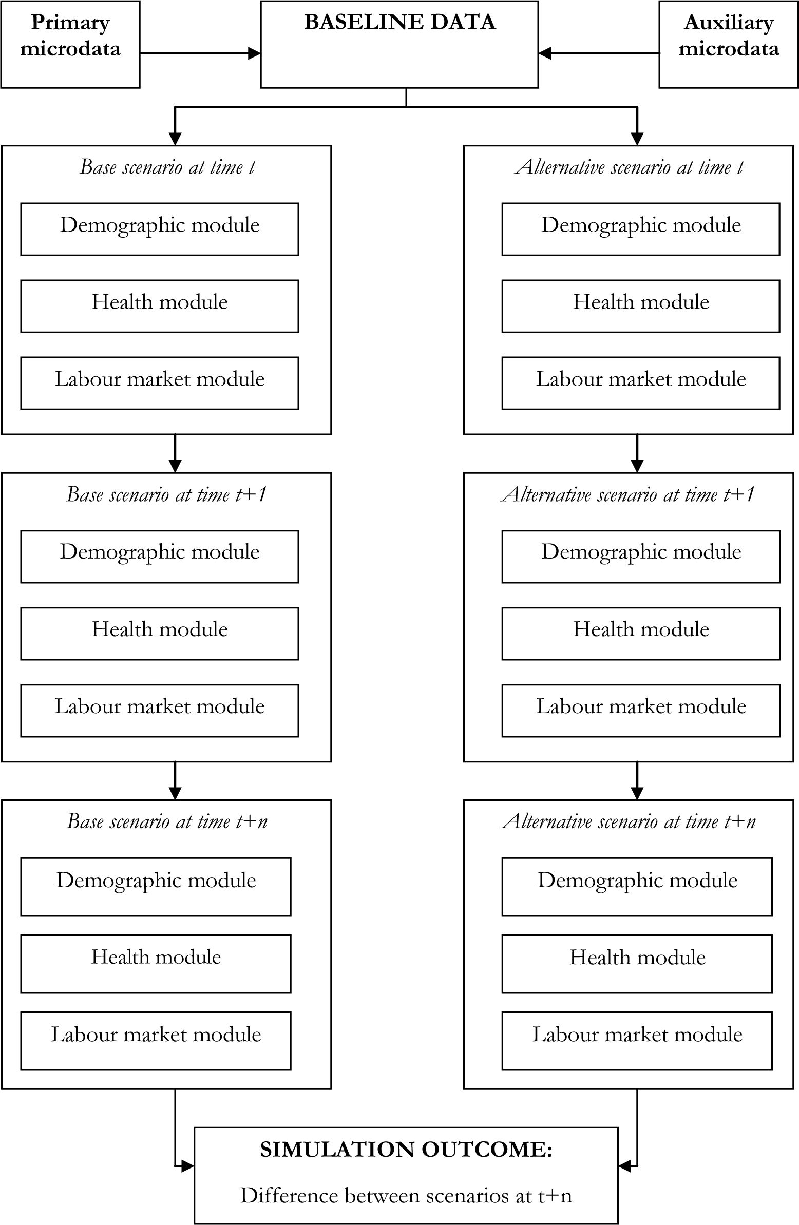
Discrete-time dynamic microsimulation models are typically structured on a modular basis where events are usually represented as a set of univariate processes that follow a hierarchical order. This structure is represented in Figure 1.
The figure shows the starting point of a dynamic microsimulation model, the baseline dataset, the modules used to simulate individual events (in this stylised example, demographic, health and labour market modules) and the outcome produced by the simulation; here the difference in the trajectories between a baseline scenario and an alternative under evaluation.
A fundamental component of any dynamic microsimulation model is its baseline dataset. This is usually composed of a main source, based on individual records taken from survey or administrative data, augmented with information imported from additional sources, using imputation or matching techniques. The rationale behind the use of multiple sources of data is often to fill information gaps in the primary data source or simply to integrate external information. Ultimately, the essential requirement for a baseline dataset is for it to be representative of the population relevant for the policy being simulated (Martini & Trivellato, 1997).
In a discrete-time setting, all individuals at a particular time period t are at risk of experiencing a series of events. The occurrence and timing of each event are established according to the Markov chain Monte Carlo rules outlined earlier. Depending on the focus of the model, modules and events may differ. However, the majority of discrete-time dynamic microsimulation models include demographic events (such as birth, mortality, household formation and dissolution and more rarely immigration), education and labour market-related events (e.g. modules that “attach” a degree to each individual and subsequently consider transitions into and out of as well as within the labour market) and less commonly health events, usually in the form of a stylised health status (for example, a binary measure of individual health status, being in good health or ill-health). Richer dynamic models might also contain modules that compute labour earnings, non-labour income, expenditures as well as reproducing the tax and social security systems of a specific country3. The baseline dataset modified by the transitions incurred by individuals at the end of a time period t becomes the input dataset for the following time period, t + 1. This is repeated until the entire dynamic simulation cycle is complete (i.e. until the last time period considered is reached).
An essential feature of a typical discrete-time dynamic microsimulation model is the hierarchical nature of the events represented. The sequence of events within each time period is established a priori by the model builder. Hence, the sequence of causal relationships between key events within an individual's life is pre-determined. Although this modelling strategy allows the researcher to control the consequence of changes within the chain of events, ignoring the potentially numerous endogeneity issues could seriously hamper the reliability of the model's results.
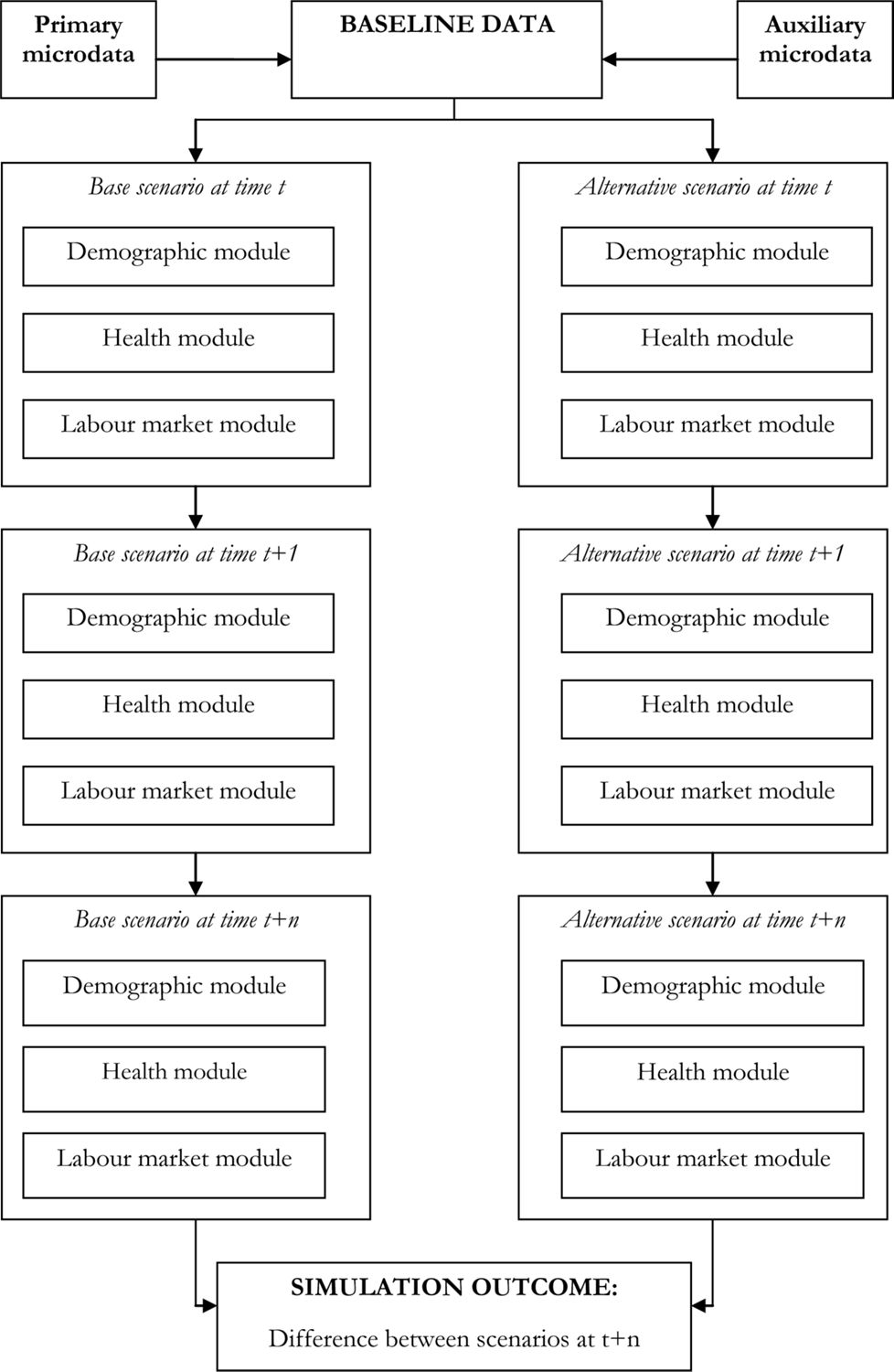
Structure of a typical discrete-time dynamic microsimulation model4.
2.3.2 Continuous-time dynamic microsimulation mode
Dynamic microsimulation can be implemented in continuous-time using duration models. In this framework, the variable of interest is the time to occurrence of an event (in this case, the time to a transition between an origin state and a destination state). Within this setting, a central mechanism that governs the timing of events is the concept of the inverse distribution function or quantile function. While a distribution function transforms a real number into a probability, the quantile function translates a probability into a real number (Willekens, 2006, 2009). In continuous-time dynamic microsimulation models, the quantile function is used to transform the probability of a transition from one state to another into a real number that represents the time to an event.
In continuous-time duration models, the time to an event T can be considered a random variable with the following cumulative distribution function (cdf):
The cdf represents the probability that the duration spell length is less than t in the interval from 0 to t (i.e. the probability that the transition between two states occurs in the period between 0 and t). The probability that the duration equals or exceeds t is defined by the survivor function:
The concentration of events along the time axis is given by the density function that is the slope of the survivor function expressed as follows:
The instantaneous rate of leaving a state conditional on survival to time t is given by the hazard function that can be expressed by:
The cumulative hazard function (or integrated hazard function) can be obtained by integrating the hazard rate at each instant in time:
The timing of the transition for an individual i is given by G(ri) where ri is a random value drawn from a uniform distribution in the interval [0,1] and G is the inverse distribution function of T, i.e. G = F−1(t). That is, the inverse distribution function or quantile function is used to map the realisation of the random draw into a real number t which indicates the timing of the transition. Hence, in the context of continuous-time dynamic microsimulation, the decision rule that is used to set the timing of an event entails two stages. First, a random number ri is drawn from a uniform distribution U ~ U[0,1]. Second, a quantile function of the probability distribution F(t) is used to convert this number ri into a real value of t.5
An example: simulating the time to transitions
As an example, we consider the simulation of the time to transition between different states produced using a Cox proportional hazard model, a widely used duration model (Bender et al., 2005). The Cox proportional hazard model can be defined through its hazard function:
where t is time, X is a vector containing a set of covariates that define a series of individual socioeconomic characteristics, ϕ is a vector of regression coefficients and h0 is the baseline hazard function (i.e. the hazard function in the absence of covariates, X=0). The survival function of the Cox proportional hazard model can be written as follows:
where H0 is the cumulative baseline hazard function. The distribution function of this model is:
Let r be a random number drawn from a uniform distribution U ~ U[0,1]. Then, the simulated time to transition T is produced using the inverse or quantile function of the Cox proportionaI hazard model that takes the following form:6
Accordingly, the simulated time to transition depends on a constant transition rate and a set of covariates. It should be noted that the Cox hazard model is not restricted to the exponential distribution and that a set of alternative survival time distributions can be used to generate simulated times to transition using Cox hazard models (for an overview, see Bender et al. 2005).
The individual life-cycle in continuous-time dynamic microsimulation modelling
In continuous time dynamic microsimulation the life-cycle of an individual can be modelled in two alternative ways (Willekens, 2009). One possibility is to simulate the entire life-cycle of an individual until the event death before starting the simulation of the life-cycle of another individual. For each individual separate times to transitions are simulated for competing events (e.g. demographic transitions, labour market transitions, transitions between different health states, etc.). The first state transition to occur is established by choosing the shortest time to transition.
An alternative is to employ discrete-time duration analysis and model segments of an individual life-cycle. The procedure consists of breaking down the continuous time frame into a series of discrete spells and considering the simulation of a set of events (transitions) within these spells. The length of the spells can vary according to the specific needs of the modeller but most applications use spell lengths of one year (Willekens, 2009). In this framework, transitions from one state to another occur by comparing the simulated time to transition for each specific event with the length of the time spell. For example, if we consider spells of the length of n years and a simulated time to transition, t, the transition occurs during the first spell n if the simulated time to transitions is less than n, (t < n). This framework also accounts for repeatable events (i.e. events that can occur more than once such as child birth, labour market and health transitions). Assuming that an event is repeatable and its first occurrence is at t1 if t1 < n, the event occurs a second time during the same spell if a second draw of a random number from the uniform distribution U ~ U[0,1] generates a simulated time to transition t2 that is less than or equal to n – t1 (t2 ≤ n – t1). As a result, the event occurs at time t1 + t2.7
Modelling multiple transitions in continuous-time dynamic microsimulation
The majority of continuous-time dynamic microsimulation models aim to model multiple transitions among a number of states. This translates into extending the framework presented above into a multiple hazard setting (Cameron and Trivedi, 2005). In this context, the basic competing risks model (CRM) offers a suitable way of modelling the time to transition between one state of origin and one of a series of competing destination states.8 Competing risks models assume that a latent duration, tj, exists for each possible destination state (or risk) j (1,....,m). In the absence of other risk factors that might cause the end of the spell to occur sooner, tj can be interpreted as the spell duration for each possible destination j. In this setting, the observed duration T is the minimum (or shortest) duration tj:
And the corresponding simulated destination state, r, is:
The distribution of tj can be modelled through its hazard function, hj, that defines the hazard rate of the jth type of failure (or transition into the destination state j). In the case of independent risks, the hazard function can be written as:
where Xj is a destination-specific vector of exogenous covariates. Provided that the event transition into destination state j has not already occurred, the hazard rate is the product of the rate of transition in the interval Δt and the probability of transiting into destination j.
Willekens (2009) highlights two approaches to model time to transition and destination states in multiple state continuous-time dynamic microsimulation. The first method simulates the time to transitions for every possible destination state. The shortest time to transition determines the actual time to event to that destination. This method is applied in two models developed at Statistics Canada, LifePaths, a dynamic microsimulation model of Canadian individuals and households, and POHEM (Population Health Model), a dynamic microsimulation of diseases and risk factors within the Canadian population.9 An alternative method employs two random draws, one to define the time to transition and the other to determine the destination state. The time to transition is simulated drawing a random number from an exponential distribution while the destination state is simulated using a draw from a uniform distribution in a fashion similar to that described earlier.
Discrete-time versus continuous-time dynamic microsimulation modelling
Several authors have discussed the relative merits of discrete-time versus continuous-time dynamic microsimulation modelling (Zaidi & Rake, 2001; Spielauer, 2007; Willekens 2009). Zaidi & Raike (2001) suggest that in principle a continuous-time framework should be preferred because it allows for intermediate (i.e. less than a year) transitions as well as enhancing the capacity to account for the interdependency and simultaneity of the multiple events modelled. However, the authors make the valid point that the majority of data available for microsimulation are collected on an annual basis making the choice of a discrete-time model that operates with annual probabilities a natural one. Further, Zaidi and Rake emphasise the possibility to model certain events using shorter time periods within a discrete-time setting, for example using monthly transitions. In his review of dynamic microsimulation models, Spielauer (2007) also appears to favour the use of continuous and pseudo-continuous (monthly steps) dynamic microsimulation. More recently, Willekens (2009) suggests that continuous-time dynamic microsimulation modelling overcomes three fundamental problems that are intrinsic in the use of discrete-time modelling. These are the possibility of determining precise sequences of events (transitions); the measurement of the exact duration/length of events and the capacity to model multiple transitions during the same time interval.
2.4 Validation
Predictions from dynamic microsimulation models must be considered credible in order to be accepted and used by both modellers and policy-makers. The credibility of a dynamic microsimulation model is based on its capacity to reproduce observed data or known benchmarks such as official population projections. Accordingly, an important aspect of dynamic microsimulation modelling is the validation of results produced by the simulation exercise. Interestingly, the applied literature has devoted little attention to validation procedures and the quantification of uncertainty around model predictions (Wolf, 2001; Klevmarken, 2002). Moreover, among practitioners there is currently no apparent consensus on what constitutes best practice. In the majority of applications, discrepancies between simulation outputs and some external benchmark are often resolved using alignment techniques. In general, alignment consists of adjustment of the simulation output in order to reflect the expected proportion of certain events in a population. Alignment methods applied to dynamic microsimulation have significantly evolved in the past few years and vary widely (Morrison, 2006). In the case of a hierarchical or recursive model such as the one depicted in Figure 1 of Section 2.3.1, a “piece-meal” validation procedure can be used (Klevmarken, 2002) where validation is performed separately for each sub-model. A comprehensive list of alignment methods can be found in Morrison (2006). For an illustration of the various validation methods applied to two different dynamic microsimulation models, DYNACAN and APPSIM, readers should refer to Morrison (2008) and Kelly and Percival (2009), respectively.
Pudney and Sutherland (1994) and Klevmarken (1998) identify three sources of uncertainty around the predictions produced by microsimulation models. These are classic sampling error, Monte Carlo errors and parameter uncertainty. Sampling error is simply the error linked to the use of a sample rather than the entire population to build the initial or base dataset. Monte Carlo errors are associated with the use of a particular set of random draws in the stochastic process that generates individual trajectories. Klevemarken (1998) suggests dealing with Monte Carlo variation by taking a high number of random draws and further proposes the use of bootstrapping techniques to account for parameter uncertainty.
3. Dynamic microsimulation and health
Existing dynamic microsimulation models have been extensively used to project populations over time, to design and evaluate public policies and to investigate income inequality and its distribution. Although a number of dynamic microsimulation models include health-related components, health is rarely the central focus of the analysis. Following O’Donoghue’s (2001) classification between multi-purposes versus special-purpose microsimulation models, we can distinguish between dynamic microsimulation models that are not specifically designed to represent health-related aspects and models explicitly centred on health and health related policies.
3.1 Multi-purposes models
Within the multi-purpose dynamic microsimulation models, health-related aspects are often included in a fairly rudimentary way. Models account for health, usually defined through disability and mainly used to inform social security benefits, institutionalisation, or to determine the need for health care and, in some cases, to project health care expenditure and usage.
DYNAMOD, the Dynamic Microsimulation Model of the Australian population (King et al., 1999) and CAPP_DYN, the Italian dynamic microsimulation model developed by the Centre for Analysis of Public Policies (Mazzaferro & Morciano, 2008), include disability as a proxy for individual health status. INAHSIM, the Integrated Analytical Model for Household Simulation for the Japanese population (Inagaki, 2008) and SAGE (Simulating Social Policy in an Ageing Population), a dynamic microsimulation model for England (Evandrou et al., 2001) use health dichotomised into two categories: “good health” and “ill-health”.10 DYNASIM3 (the third version of the Dynamic Simulation of Income model for the US) includes individual health measured by the number of limitations on activities of daily life (ADLs) as well as by limitations on instrumental activities of daily living (IADLs). It also includes events such as the onset and recovery of disability and institutionalisation (Favreault & Smith, 2004). MOSART, the dynamic microsimulation model for Norway, includes a number of health events: moving in or out of old age care institutions, rehabilitation, disability and public disability pensions (Fredrisken, 2003). Further aspects of health are also included in the Cornell Dynamic Population Microsimulation model (CORSIM) for the US, including risk factors (smoking, alcohol and sugar consumption, diabetes), disability status, institutionalisation as well as disability insurance and dental conditions, services and expenditures (Strategic Forecasting, 2002). SESIM (Bolin et al., 2007), the dynamic microsimulation model of the Swedish Ministry of Finance, and APPSIM (Lymer, 2009), the Australian Population and Policy Simulator, focus on the consequences of ageing and model health status, health care expenditure and health service usage.11 The HARDING model for Australia, a cohort dynamic microsimulation model, also models health service usage as well as health expenditure (Harding et al., 2002). However, it does not model individual health status in itself.
3.2 Models focused on health
A limited but growing number of dynamic microsimulation models are centred on health. Among these models, the aspects of health considered and the methods used vary widely depending on the models’ specific objectives and the type of health interventions under scrutiny. In this section, we briefly describe objectives, main modelling features and, when the information is available, validation and findings of a series of health-dedicated microsimulation models.
The majority of health-focused dynamic microsimulation models attempt to project and estimate long-term health care costs and the incidence of disability and chronic conditions. Van Sonsbeek and Gradus (2006) employ a combination of dynamic ageing and behavioural microsimulation modelling to predict the likely impact of the 2006 regime change of the disability benefit scheme in the Netherlands. The authors find that the introduction of the proposed system would decrease the number of individuals relying on disability benefits and would increase labour market participation. The plausibility of the results produced by this model is tested by comparing them with other long-term forecasts based on data from the Dutch Benefit Administration Office. Lymer et al. (2009b) built CAREMOD, a spatial microsimulation model for the projection of the need for elderly care services at small area level. Using a series of re-weighting techniques on both survey data on disability and census data, CAREMOD produces small area level forecasts of the prevalence of disability, care needs and characteristics of the older population in New South Wales, the largest state in Australia. Various alignment methods to external sources of data were used for the validation of the model and particular attention was devoted to the reliability of the simulated small area estimates of rare events such as severe disability. Schofield et al. (2009) recently developed Health&WealthMOD, a microsimulation model concerned with the impacts of health and disability on labour force participation, income and the Australian government’s revenues and expenditures. The model combines survey data on disability with data on income and taxes produced by STINMOD together with information on future individual wealth from DYNAMOD, two of NATSEM’s microsimulation models. Early applications of Health&WealthMOD quantify the impact of lost taxation revenue and increases in government transfer payments due to mental health conditions (Schofield et al., 2011a) and long-term illness (Schofield et al., 2011b).
Dynamic microsimulation methods have been used recently to project the future impact of specific chronic conditions. Sassi et al. (2009) employ the Chronic Disease Prevention Model (CDP), by implementing dynamic ageing and various imputation methods, to assess the cost-effectiveness and distributional impact of obesity-related interventions in selected OECD countries. The authors present a series of findings and conclude that although most of the preventive interventions evaluated appear to have favourable cost-effectiveness ratios, they might not always reduce total health expenditure when the costs of diseases affected by diet, obesity and physical activity are considered. Sassi et al. conduct a sensitivity analysis using confidence intervals associated with individual parameter estimates as well as running a number of Monte Carlo simulations with different distributions of input parameters. A prototype of a model for the analysis of the incidence and progression of type II diabetes and cardiovascular diseases, HealthAgeingMod, is described in Walker et al. (2010). The model combines chronic disease progression models to a population-wide microsimulation model that projects the base-year population through re-weighting techniques. The model is also designed to use standard cost-benefit and cost-effectiveness methods to assess the impact of a series of simulated policy options. In this case, the validation of the prototype model was conducted through the alignment to external benchmarks.
Finally, other microsimulation models have been used to analyse the impact of government pharmaceutical benefits schemes. For example, Abello et al., (2008) use various imputation and re-weighting methods to analyse the distributional effect of the Australian Pharmaceutical Benefit Scheme (PBS). Their results highlight that the scheme is highly progressive with two-fifth of total PBS outlays being directed at the poorest-one fifth of the population. Abello et al. also illustrate the usefulness of statistical matching and the use of complementary sources of data to overcome data limitations in their main base file.
The following section focuses on a more detailed description of two models, the Population Health Model (POHEM) and the Future Elderly Model (FEM) which are currently among the most comprehensive dynamic microsimulation models dedicated to health. Together with the HealthAgeingMod prototype model earlier described, POHEM is one of the few existing models that simultaneously accounts for the progression and interactions of multiple health conditions. FEM is a leading example of a model that can simulate a number of potential health breakthroughs together with government health expenditure. Both models have the flexibility of being used to evaluate a variety of policy interventions.
3.2.1 Population health model
POHEM (Population Health Model) is a continuous-time dynamic microsimulation model designed to represent the lifecycle dynamics of the Canadian population.12 The model focuses on the evolution and interactions of a set of specific diseases and risk factors. POHEM also includes individual-level data on health care costs and utilisation together with a measure of health-related quality of life, the Health Utility Index Mark 3 (HUI3) (Grootendorst, 2000). Initially developed by Statistics Canada as a sub-model of the microsimulation model Lifepaths, POHEM integrates data from different sources on heart disease, diabetes, osteoarthritis, different types of cancer (lung, breast and colorectal cancer) and risk factors such as smoking, body mass index, cholesterol, blood pressure and mortality. Starting from this comprehensive baseline dataset, the model employs continuous-time dynamic microsimulation techniques to age the initial population forward in time and to model the onset and evolution of disease, co-morbidities and the influence of risk factors.
The baseline dataset: integrating different sources
The baseline dataset of POHEM combines data drawn from a multiplicity of sources. These include the Canadian Community Health Service (CCHS), the Statistics Canada’s census projections, the National Population Health Survey (NPHS), the Canadian Heart Health Survey (CHHS), the Health Person Oriented Information (HPOI), the Registered Persons Database (RPDB) and the British Columbia Linked Hospital Database (BCLHD).13 Each source of data was employed for a specific purpose. The CCHS is a cross sectional survey started in 2000-2001 with an initial sample of 131,535 individuals, representative of the Canadian household population aged 12 and over. The survey was used to define the initial population that is projected forward in time by the simulation model. Statistics Canada’s census projections were employed to inform the projections of new births and immigrants in the simulation. Data on Body Mass Index and cigarette consumption were integrated using information drawn form the NPHS, a longitudinal survey started in 1994-1995 with an initial sample of 17,276 Canadian individuals. Blood pressure, total cholesterol and high density lipid count were modelled using data contained in the Canadian Heart Health Survey (CHHS), a cross-sectional survey of 23,129 individuals conducted between 1986 and 1992. Statistics Canada’s HPOI includes hospital morbidity records drawn from the Canadian Institute for Health Information’s (CIHI) general records and was used both to improve the quality of the morbidity files and to derive rates of incidence of acute myocardial infarction. The RPDB dataset links the CIHI’s morbidity records with the vital statics for Ontario from 1988 to 2002 and was used to model survival times following different types of acute myocardial interventions. Finally, data on visits to health professionals and hospital admissions covered by the Medical Services Plan of British Columbia were included in the baseline data of the BCLHD.
Modelling approach: continuous-time dynamic microsimulation
In order to model the life-cycle dynamics of diseases and risk factors, POHEM makes use of continuous-time dynamic microsimulation modelling techniques. Microsimulation is employed to model the onset, progression and cessation of disease as well as the ageing process of the population. The time to incidence of each disease is established according to the general methodology depicted in Section 2.3. In this case, random draws generated through Monte Carlo simulations are converted into time to transitions using the inverse function of piecewise Weibull proportional hazards models. Co-morbidities are modelled as multiple hazards where the shortest time to transition determines the first transition to occur. POHEM is organised on a modular basis and contains a sub-model for each disease and risk factor. Below, we provide further details for each sub-model.
Disease-specific sub-models
POHEM contains four disease sub-models: a heart diseases model, a diabetes model, an osteoarthritis model and a cancers model.14 The heart disease sub-model simulates the incidence of acute myocardial infarction (AMI) using data on socioeconomic characteristics and risk factors from various sources (the Canadian Community Health Service, the National Population Health Survey and The Canadian Heart Health Survey). The Framingham risk incidence function (Wilson et al., 1998) is used to predict the incidence of AMI according to individual sociodemographic characteristics such as age, gender, region of residence and risk factors such as total cholesterol, blood pressure, smoking and body weight. Once the initial prevalence of risk factors is established, the model projects individuals through time and produces projections for episodes of acute myocardial infarction for each individual until death. Data produced from this sub-model are subsequently used to inform the other sub-models of POHEM.
The diabetes sub-module is based on the Diabetes Population Risk Tool (DPORT), a diabetes risk incidence model developed using data from the National Population Health Survey, the Ontario Diabetes Database and the state of Ontario mortality rates. This model produces diabetes type II incidence rates according to a series of socioeconomic determinants (age, gender, education, income, ethnicity, geographical area) and risk factors (alcohol, smoking, blood pressure, obesity, physical activity). The sub-model also produces incidence rates of different diseases resulting from type II diabetes such as coronary heart disease, stroke, diabetic retinopathy, kidney diseases, etc. The incidence rates produced by the diabetes model are employed in the other sub-models.
The osteoarthritis model measures the prevalence and incidence of osteoarthritis using data from the Canadian Community Health Service and the National Health Population Survey (Kopec et al., 2009). This model includes the possibility of modelling changes in health-related quality of life using the Health Utility Index Mark 3 (HUI3). Finally, the cancers sub-model produces the incidence and progression of lung, breast and colorectal cancers.
Risk factors sub-models
POHEM includes three risk factor sub-models: smoking, the evolution of body mass index (BMI) and blood-related risk factors (total cholesterol, high density lipid count (HDL) and blood pressure). Within the smoking sub-model, smoking status (being a regular smoker or former smoker who quit within the last year or alternatively being a non-smoker) and transitions between smoking states are modelled using data from National Population Health Survey (NPHS). Transitions are based on a fourth-order Markov process and are conditional on age, gender and previous smoking status. The evolution of individual BMI is informed by a series of linear regressions of self-reported BMI estimated on data drawn from the NPHS. The set of covariates used for the BMI regression models include age, gender, region of residence, income quartile, education and previous BMI. The blood-related risk factors sub-model estimates joint probabilities of changing total cholesterol levels (among low, low-medium, medium, medium-high and high quantity of total cholesterol) and blood pressure states (optimal, normal, high-normal, hypertensive stage I, Hypertensive stage II-IV). These probabilities are derived using data from the Canadian Heart Health Survey.
Outputs
To date, POHEM has been used mainly to evaluate the costs-effectiveness of a number of disease-specific interventions. Evans et al. (1997) use POHEM to evaluate the cost-effectiveness of new combined (preoperative and postoperative) therapies on patients with non-small-cell lung cancer (NSCLC). They find that this combined treatment strategies would confer a survival advantage and would also be cost-effective. The authors tested the accuracy of these findings by varying the survival gains and the length of the hospitalisation corresponding to these interventions. Berthelot et al. (2000) also employ the model to evaluate the cost-effectiveness of alternative treatments on patients with NSCLC and conclude that chemotherapeutic treatments should be preferred to palliative and supportive care measures. In order to assess the robustness of these results, the authors use different cost-effectiveness thresholds and different hospital spell lengths for the various treatment regimes. More recently, Kopec et al. (2009) employ POHEM to model and quantify the future incidence of osteoarthritis and its effect on health-related quality of life. Results from this application are validated by comparing and aligning the simulated frequencies to a variety of external sources of data.
3.2.2 Future elderly model
The Future Elderly Model (FEM) is a demographic and economic microsimulation model developed at RAND (Goldman et al., 2004). It focuses on predicting future health care expenditures and the health status of a population of older Americans drawn from the Medicare Current Beneficiary Survey (MCBS). The model consists of three main components: a model for health care costs, a model of health status transitions and a model that predicts health characteristics of new Medicare enrolees (termed the “rejuvenation” model). FEM is used for evaluating what-if scenarios of a variety of health care interventions.
Data
FEM makes use of individual records drawn from the MCBS (1992–1998), a nationally representative dataset of Medicare beneficiaries composed of individuals who are either over 65, disabled or institutionalised. Originally developed as a longitudinal survey, the first MCBS sample was collected in 1992 and included 10,584 individuals. Since 1996, the MCBS became a rotating panel and new samples of around 10,000 individuals were introduced each year until the end of the survey in 1998. The MCBS contains self-reported information on height, weight, general health status, a set of specific health conditions (different types of cancers, heart disease, Alzheimer, stroke, diabetes, hypertension, lung-related conditions, arthritis), measures of physical limitations in performing Activities of Daily Living (ADL) and Instrumental Activities of Daily Living (IADL). The survey also includes variables on health care utilisation and expenditures obtained through self-reported information and the Medicare service use records.
Model structure
FEM comprises three main sub-modules. The first produces individual trajectories for a number of health conditions and disability statuses. A second sub-module (the rejuvenation module) ensures that the data remains representative of the population aged 65 years or over. A third sub-module projects future Medicare and total health care expenditures based on the demographic and health characteristics of the population.
Health transitions sub-module
In the first sub-module, transitions into mortality, cancers (breast, prostate, uterus, colon, bladder, lung, kidney, throat, head, brain), cardiovascular disease (angina pectoris, myocardial infarction), neurological disorder, diabetes, hypertension, ADL and facility residence (i.e. entry into a nursing home) are modelled using piecewise Gompertz proportional hazard models. Covariates include socio-demographic characteristics (age, gender, ethnicity, and education), co-morbidities and risk factors (smoking and obesity). Individual transition probabilities obtained from these models are compared with random numbers extracted from a uniform distribution [0,1]. Health transitions occur whenever the transition probabilities exceed the corresponding random draws. In FEM, all health conditions are treated as absorbing (i.e. permanent) states.
Rejuvenation sub-module
The second sub-module is designed to predict the health and disability status of the entering cohorts of Medicare patients between the years 2001 and 2030 using data on chronic disease from the National Health Interview Survey (NHIS) and information on cause-specific mortality profiles from the Vital Statistics of the United States. In this module, the prediction of the health status of the cohorts entails three main steps. First, age-specific prevalence rates are obtained for each chronic disease considered (heart disease, hypertension, cerebrovascular disease, Alzheimer, cancer, diabetes, chronic obstructive pulmonary disease) and disability status using data from the NHIS. Second, age-incidence trajectories are created combining information on successive disease prevalence and disease-specific death rates from the US Vital Statistics. Third, age-specific prevalence rates and disease-specific trajectories generated in the previous two steps are used to predict and adjust the health status of the incoming Medicare sample.15
Health expenditure sub-module
The health expenditure module aims to identify the determinants of health care expenditures among elderly Americans. In this module, Medicare reimbursements and total healthcare expenditures are predicted using OLS cost regression models. Explanatory variables include socio-demographic characteristics (age, gender, ethnicity, education, geographical area of residence), health measures (self-reported health, ADL, self-reported diseases such as cancer, heart disease, diabetes and neurological conditions as well as interactions with ADL categories and disease conditions), mortality, obesity, smoking and nursing home residency.
Scenario modelling and outputs
FEM simulates a set of potential scenarios identified by a technical expert panel (TEP).16 These simulated scenarios include potential breakthrough technologies in areas such as disease prevention, early detection and improved treatments of certain diseases but also changes in the health care system and in individuals’ lifestyles. In order to evaluate the effectiveness of these health interventions, the model compares disease prevalence rates and related costs across the baseline and simulated scenarios. Examples of applications of FEM include the simulation of alternative technological advancements in cancer treatment to project spending among the elderly through to 2030 (Battacharya et al., 2005). This exercise concludes that due to demographic changes, even inexpensive and effective technologies (including early cancer detection scenarios via improved screening technologies and new drugs treatments) may not necessarily lead to a decline in total medical spending. Goldman et al. (2005) employ FEM to assess how new medical advances (e.g. the availability of a series of devices for different heart conditions and cancer treatment technologies) would affect individuals’ health status and health care spending over the period 2000-2030. Their findings appear to suggest that most of these promising medical technologies would greatly increase spending. It is not clear how the models are validated prior to use.
4. Conclusions and discussion
Dynamic microsimulation and health
This paper has two core objectives. The first is to present an overview of microsimulation methods and applications that are relevant for the purpose of health policy evaluation. The second is to present a review of existing dynamic microsimulation models that include a health component together with the most recent and comprehensive models focused on health. Throughout the paper we have illustrated the power of dynamic microsimulation as a valid tool for the evaluation of health policies and hope we have made a case for the greater use of these approaches. Dynamic microsimulation offers a number of important advantages over more standard methods of ex-post policy evaluation. First, by simulating data under alternative scenarios, dynamic microsimulation allows for the evaluation of outcomes of interest prior to actual implementation of a policy. Secondly, by projecting individual socioeconomic and health trajectories over multiple periods of time, dynamic microsimulation techniques readily incorporate heterogeneity in estimated treatment effects together with the long-run effects of treatment. Finally, dynamic microsimulation can additionally be used to identify better externalities and spillovers in treatment.
From our review of models and methods it emerges that dynamic microsimulation offers a number of advantages for the purpose of evaluating health interventions. Dynamic microsimulation provides the opportunity of creating novel data sources covering a number of health conditions as well as health behaviours. Moreover, unlike any other single-disease model, microsimulation allows for modelling simultaneously the evolution and interaction of multiple diseases and risk factors together with other important individual socioeconomic characteristics such as labour market status. Allowing for comorbidities is of particular importance when simulating the evolution of an individual health status and the effects of health policies.
Another indication from our review is that the evaluation of specific types of health policies often requires the use of different microsimulation methods. Only some of the most recent and comprehensive dynamic microsimulation models of health (e.g. the Chronic Disease Prevention Model, the Future Elderly Model, HealthAgeindMod and the Population Health Model) combine different microsimulation features and are capable of simulating a variety of policy options ranging from medical treatments (e.g. new drugs or chemotherapeutic treatments) to public health reforms focused on lifestyle changes (e.g. diet and exercise). However, the majority of the existing health-focused microsimulation models employ static ageing and re-weighting techniques mainly to project the future prevalence of disability and to evaluate disability-related policy interventions.
Limitations of the approach
As has been noted in previous studies, a fundamental limitation concerning the use of dynamic microsimulation is the difficulty and time required to collect and combine different sources of data together with the wide range of expertise required to construct meaningful models (Spielauer, 2007). A clear trade-off between model complexity and comprehensiveness versus time appears to be evident. Further, although the most recent health studies produced using dynamic microsimulation techniques propose a series of validation strategies, there are currently no common standards for the validation of model projections and predictions and the quantification of uncertainty.
It is also important to stress that the output of any microsimulation model relies on a particular set of assumptions regarding the behaviour of the micro-units represented. These assumptions need to be credible for the microsimulation exercise to have validity. Further, while estimates of behavioural microsimulation models have the advantage of being grounded on economic theory, they tend to be policy-specific and difficult to extend to alternative contexts. Dynamic microsimulation models that project the characteristics of a population over time usually include the simulation of a series of interacting micro-processes such as demographic, labour market and health dynamics. The way in which these processes interact with each other represents the core of a dynamic microsimulation model. These interactions are however rarely justified using structural models. That is, dynamic microsimulation models often include very limited behavioural components.
Potential research avenues
One of the key challenges facing the future development of dynamic modelling is the incorporation of credible structural microeconomic models capable of taking into account the various behavioural components of the simulation exercise. In particular, the fundamental challenge that modellers have to face is the choice of an appropriate theoretical framework to define agents’ dynamic optimising behaviour. In the context of both the analysis of the dynamics of health and the evaluation of health policies, Grossman’s (1972) seminal work on health capital and the demand for health and its related literature (for example Dardanoni, 1986; Ried, 1998; and Forster, 2001) offer a credible foundation. Ippolito’s (1981) model of lifecycle consumption of hazardous goods, Becker and Murphy’s (1988) theory of rational addiction and the more recent model of Carbone et al. (2005) on smoking, health-investment and mortality risk may be more appropriate in informing dynamic microsimulation models aimed at evaluating the efficacy of public health interventions based on reducing risky lifestyle behaviours. Ultimately the choice of a particular structural framework should be in accordance with the specific objectives of the microsimulation model but should also be amenable to the implementation of its empirical counterpart.
Footnotes
1.
It should be noted that the choice between static and dynamic microsimulation approaches is only partly due to the objectives of the analysis and that, given the complexity of dynamic microsimulation modelling (see
2.
More sophisticated models distinguish between an optimizing error and random preference heterogeneity. In this type of model, optimising errors are simply regarded as errors in perception of the alternative utilities or as unobserved alternative-specific utility factors whereas random preference heterogeneity is intended to reflect random preferences derived from unobserved individual characteristics. For a brief discussion, see Brewer et al., 2005.
3.
One of the most comprehensive discrete-time dynamic microsimulation models is the Australian Population and Policy Simulator (APPSIM) that is currently under development at NATSEM, University of Canberra. For a brief overview of the APPSIM simulation cycle, see http://www.canberra.edu.au/centres/natsem7research-models/projects_and_models/appsim
4.
This graph is based on Graph 1 in Martini and Trivellato (1997).
5.
In the majority of applications, the distribution F(t) is assumed to be either exponential, Gompertz or Weibull. If the time to a transition event follows an exponential distribution, then transitions are assumed to occur at a constant rate. In case of a Gompertz distribution, the transition rate changes exponentially with duration while with a Weibull distribution the transition rate varies with duration following a power function of duration.
6.
It should be highlighted that in equation (17), H0 can be inverted if h0(t) > 0 for all t.
7.
For an example, see Willekens (2009).
8.
For a fuller explanation of competing risks models, see Chapter 19 pp.642-648 of Cameron and Trivedi (2005) and Mealli and Pudney (1996). In this section, we broadly follow these expositions.
9.
10.
The Economic and Social Research Council (ESRC) Research Group for Simulating Social Policy in an Ageing Society (SAGE) was established in November 1999 with funding from the ESRC. It was jointly located within the Social Policy Department at LSE, the Institute of Gerontology at King’s College London and the School of Social Science at the University of Southampton.
11.
The health module of the APPSIM model is currently under construction. The information on its main features is drawn from Lymer (2009).
12.
A general overview of POHEM can be found in the POHEM page at the Statistics Canada website (http://www.statcan.gc.ca/microsimulation/pohem/pohem-eng.htm). The information contained in this section on structure, data and mechanics of POHEM was obtained combining a variety of sources: Evans et al. (1997), Berthelot et al. (2000), Will et al. (2001), Kopec et al. (2009), the LifePaths microsimulation model overview (http://www.statcan.gc.ca/microsimulation/pdf/lifepaths-overview-vuedensemble-eng.pdf) and a series of presentations on POHEM that are freely available at the website of the International Microsimulation Association (IMA) (http://www.microsimulation.org/IMA/Ottawa_2009.htm).
13.
This list of datasets includes only the main sources of data used in POHEM and is not meant to be comprehensive.
14.
The structure of the model is here illustrated in a simplified way. For more details on the main components of POHEM, the different sub-modules and their state of development see the “Overall person life flow” scheme contained in any of the POHEM-related presentations given at the second General Conference of the International Microsimulation Association (IMA) (http://www.microsimulation.org/IMA/Ottawa_2009.htm). Part of the overall POHEM structure is also illustrated in Kopec et al. (2009).
15.
For a detailed description of the statistical models used in each of these phases, see Goldman et al. (2004), Chapter 7, pp. 72–83.
16.
The panel was formed by social scientists and experts on cardiovascular diseases, biology of ageing and cancer and neurological diseases. For a full list of members of this panel, see Goldman et al., (2004), Appendix B, p. 194, and Appendix C, pp. 202–203.
References
-
1
Enhancing the Australian National Health Survey Data for Use in a Microsimulation Model of Pharmaceutical Drug Usage and CostJournal of Artificial Societies and Social Simulation, 11, 3-2.
-
2
The Wanless report and decision-making in public healthJournal of Public Health 27:133–134.
-
3
Models for Retirement Policy Analysis, Report to the Society of ActuariesSchaumburg, Illinois Society of Actuaries (SOA).
-
4
The choice of paid childcare, welfare, and labor supply of single mothersLabour Economics 10:133–147.
-
5
What do we learn about tax reform from international comparisons? France and BritainEuropean Economic Review 32:343–352.
-
6
Microsimulation of Social Policy in the European Union: Case Study of a European Minimum PensionEconomica 69:229–243.
-
7
Orcutt’s vision, 50 years on. LABORatorio R. Revelli. Center for Employment Studies Working Paper No. 65Orcutt’s vision, 50 years on. LABORatorio R. Revelli. Center for Employment Studies Working Paper No. 65.
- 8
-
9
Generating survival times to simulate Cox proportional hazard modelsStatistics in Medicine 24:1713–1723.
-
10
Decision Framework for Chemotherapeutic Interventions for Metastatic Non-Small-Cell Lung CancerJournal of the National Cancer Institute 92:1321–1329.
-
11
Technological Advances In Cancer And Future Spending By The ElderlyHealth Affairs - Web Exclusive W5-R53–W5-R66.
-
12
The Labour Supply, Unemployment and Participation of Lone Mothers in In-Work Transfer ProgrammesEconomic Journal 107:1375–1390.
-
13
Microsimulation as a tool for evaluating redistribution policiesJournal of Economic Inequality 4:77–106.
-
14
Did Working Families’ Tax Credit work? The final evaluation of the impact of inwork support on parents’ labour supply and take-up behaviour in the UK. Inland Revenue Working Paper 2. HM Revenue and CustomsDid Working Families’ Tax Credit work? The final evaluation of the impact of inwork support on parents’ labour supply and take-up behaviour in the UK. Inland Revenue Working Paper 2. HM Revenue and Customs.
-
15
Did working families’ tax credit work? The impact of in-work support on labour supply in Great BritainLabour Economics 13:699–720.
-
16
The Effect of Financial Incentives on Labour Supply: Evidence for Lone Parents from Microsimulation and Quasi-Experimental EvaluationFiscal Studies 29:285–325.
-
17
Family Labour Supply and Taxes in IrelandTechnical Report, Economic and Social Research Institute (ESRI), WP078.
-
18
The impact of comparable policies in European countries: Microsimulation approachesEuropean Economic Review 41:627–633.
- 19
-
20
Problems and Prospects for Dynamic Microsimulation: A Review and Lessons for APPSIM. NATSEM Discussion. Papers no.63University of Canberra: National Centre for Social and Economic Modelling (NATSEM).
-
21
New International Poverty Reduction StrategiesEvaluating poverty reduction policies. The contribution of microsimulation techniques, New International Poverty Reduction Strategies, London, Routledge Books.
-
22
Microsimulation as a tool for the evaluation of public policies: methods and applicationsGrowth, Distribution and Poverty in Madagascar: Learning from a Microsimulation Model in a General Equilibrium Framework, Microsimulation as a tool for the evaluation of public policies: methods and applications, Madrid, Fundación BBVA.
- 23
-
24
Behavioural Microsimulation with Labour Supply ResponsesJournal of Economic Surveys 16:1–39.
-
25
Discrete Hours Labour Supply Modelling: Specification, Estimation and SimulationJournal of Economic Surveys 19:697–734.
- 26
-
27
Microsimulation and Public PolicyA Case Study of Unemployment Scheme for Belgium and The Netherlands, Microsimulation and Public Policy, Amsterdam, North Holland.
-
28
The Impact of Economic Policies on Poverty and Income Distribution: Evaluation Techniques and ToolsAnalyzing the Incidence of Public Spending, The Impact of Economic Policies on Poverty and Income Distribution: Evaluation Techniques and Tools, Oxford, Oxford University Press.
-
29
Overview of DYNACAN: a full-fledged Canadian actuarial stochastic model designed for the fiscal and policy analysis of social security schemes. Report for the International Actuarial AssociationOverview of DYNACAN: a full-fledged Canadian actuarial stochastic model designed for the fiscal and policy analysis of social security schemes. Report for the International Actuarial Association.
-
30
Cost of combined modality interventions for stage III non-small-cell lung cancerJournal of Clinical Oncology 15:3038–3048.
- 31
-
32
Overview of the Population Health Model (POHEM)Overview of the Population Health Model (POHEM), Statistics Canada.
-
33
The meaning of death: some simulations of a model of healthy and unhealthy consumptionJournal of Health Economics 20:613–638.
-
34
The MOSART Model - A Short technical DocumentationThe MOSART Model - A Short technical Documentation, Paper presented at the International Conference on Population, Ageing and Health Canberra.
- 35
-
36
Evaluating the public health impact of health promotion interventions: the RE-AIM frameworkAmerican Journal of Public Health 89:1322–1327.
-
37
Consequences Of Health Trends And Medical Innovation For The Future ElderlyHealth Affairs - Web Exclusive W5-R5–W5-R17.
-
38
Health Status and Medical Treatment of the Future Elderly. echical Report N 169 Prepared for the Centers for Medicare and Medicaid Services R and CorporationHealth Status and Medical Treatment of the Future Elderly. echical Report N 169 Prepared for the Centers for Medicare and Medicaid Services R and Corporation.
-
39
Educational policies and poverty reduction in Cöte d’IvoireJournal of Policy Modeling 27:231–247.
-
40
Health Utilities Index Mark 3: Evidence of Construct Validity for Stroke and Arthritis in a Population Health SurveyMedical Care 38:290–299.
-
41
On the Concept of Health Capital and the Demand for HealthThe Journal of Political Economy 80:223–255.
-
42
A Conceptual Framework to Measure Performance of the Public Health SystemAmerican Journal of Public Health 91:1235–1239.
-
43
Challenges and Opportunities of Dynamic Microsimulation Modelling. Online Conference Paper - CP 107
-
44
The Lifetime Distributional Impact of Government Health OutlaysAustralian Economic Review 35:363–379.
-
45
Micro Data, Heterogeneity, and the Evaluation of Public Policy: Nobel LectureJournal of Political Economy 109:673–748.
- 46
- 47
-
48
Projections of the Japanese Socioeconomic Structure Using a Microsimulation Model (INAHSIM)The Review of Socionetwork Strategies 2:25–41.
- 49
-
50
Structural Model of Multiple Welfare Program Participation and Labor SupplyInternational Economic Review 39:553–589.
-
51
National Centre for Social and Economic Modelling (NATSEM)Technical paper No. 19, National Centre for Social and Economic Modelling (NATSEM), University of Canberra.
-
52
DYNAMOD-2: An Overview. Online Techincal Paper No. 19National Centre for Social and Economic Modelling (NATSEM).
-
53
Behavioral Modeling in Micro Simulation Models. A Survey. Working Paper No. 31Uppsala University, Department of Economics.
-
54
Statistical inference in micro-simulation models: incorporating external informationMathematics and Computers in Simulation 59:255–265.
-
55
Simulating the future of the Swedish baby-boom generations. Working Paper No. 26Uppsala University, Department of Economics.
-
56
Development of a population-based microsimulation model of osteoarthritis in CanadaOsteoarthritis and Cartilage In press.
-
57
Discrete choice models of labour supply, behavioural microsimulation and the Spanish tax reformsJournal of Economic Inequality 6:247–273.
-
58
New Methods for Analyzing Active Life ExpectancyJournal of Aging and Health 10:214–241.
-
59
Population ageing and health outlays: assessing the impact in Australia during the next 40 years2nd General Conference of the International Microsimulation Association.
-
60
Predicting The Need For Aged Care Services At The Small Area Level: The CAREMOD Spatial Microsimulation ModelInternational Journal of Microsimulation 2:27–42.
-
61
The Role of Survey Data in Microsimulation Models for Social Policy AnalysisLABOUR 11:83–112.
-
62
Center for the Analysis of Public Policies (CAPP) Paper No. 48Center for the Analysis of Public Policies (CAPP) Paper No. 48, University of Modena and Reggio E., Faculty of Economics “Marco Biagi”.
-
63
Dynamic Microsimulation: A Methodological SurveyBrazilian Electronic Journal of Economics, 4, 2.
-
64
A New Type of SocioEconomic SystemThe Review of Economics and Statistics 39:116–123.
- 65
- 66
-
67
Evidence for public health policy on inequalities: 1: The reality according to policymakersJournal of Epidemiology and Community Health 58:811–816.
-
68
Comparative dynamic analysis of the full Grossman modelJournal of HEalth Economics 17:383–425.
-
69
Statistical Matching Using Files Concatenation with Adjusted Weights and Multiple ImputationsJournal of Business & Economic Statistics 4:87–94.
-
70
Criteria for evaluating evidence on public health interventionsJournal of Epidemiology and Community Health 56:119–127.
-
71
Improving Lifestyles, Tackling Obesity: The Health and Economic Impact of Prevention Strategies. OECD Health Working Papers No. 48OECD.
-
72
Health&WealthMOD: A Microsimulation Model Of The Economic Impacts Of Diseases On Older WorkersInternational Journal of Microsimulation 2:58–63.
-
73
The personal and national costs of mental health conditions: impacts on income, taxes, government support payments due to lost labour force participationBMC Psychiatry, 11, 72.
-
74
Economic impacts of illness in older workers: quantifying the impact of illness on income, tax revenue and government spendingBMC Public Health, 11, 418.
-
75
The Impact of Economic Policies on Poverty and Income Distribution: Evaluating Techniques adn ToolsEstimating the Indicence of Indirect Taxes in Developing Countries, The Impact of Economic Policies on Poverty and Income Distribution: Evaluating Techniques adn Tools, Oxford, Oxford University Press.
-
76
Micro-simulation and Normative Policy Evaluation: An Application to Some EU Tax Benefits SystemsJournal of Public Economic Theory 7:593–622.
-
77
Dynamic Microsimulation of Health Care Demand, Health Care Finance and the Economic Impact of Health Behaviours: Survey and ReviewInternational Journal of Microsimulation 1:35–53.
-
78
Assessing the Impact of a School Subsidy Program in Mexico: Using a Social Experiment to Validate a Dynamic Behavioral Model of Child Schooling and FertilityAmerican Economic Review 96:1384–1417.
-
79
Penn Institute for Economic Research (PIER) Working Paper 06-022Penn Institute for Economic Research (PIER) Working Paper 06-022, Department of Economics, Univerisity of Pennsylvenia, 06-022.
-
80
A Microsimulation Analysis of the 2006 Regime Change in the Dutch Disability SchemeEconomic Modelling 23:427–456.
-
81
Evidence-Based Public Health: Moving Beyond Randomized TrialsAmerican Journal of Public Health 94:400–405.
-
82
Economic model system of chronic diseases in Australia: a novel approach initially focusing on diabetes and cardiovascular diseaseInternational Journal of Simulation and Process Modelling 6:137–151.
-
83
Securing good health for the whole population: Final reportEnglish Department of Health.
-
84
Canada’s Population Health Model (POHEM): a tool for performing economic evaluations of cancer control interventionsEuropean Journal of Cancer 37:1797–1804.
-
85
Bridging the micro-macro gap in population forecastingDescription of the multistate projection model (Multistate model for biographic analysis and projection), Bridging the micro-macro gap in population forecasting, the Hague, Netherlands Interdisciplinary Demographic Institute.
-
86
New Frontiers in Microsimulation ModellingContinuous-time Microsimulation in Longitudinal Analysis, New Frontiers in Microsimulation Modelling, Vienna, Ashgate.
-
87
Prediction of Coronary Heart Disease Using Risk Factor CategoriesCirculation 97:1837–1847.
-
88
The Role of Microsimulation in Longitudinal Data AnalysisCanadian Studies in Population 28:313–339.
-
89
Papers in Microsimulation Series Paper No. 4Maxwell Center for Demography and Economics of Aging, Syracuse University.
-
90
Ex Ante Policy Evaluation, Structural Estimation, and Model SelectionAmerican Economic Review 97:48–52.
-
91
Dynamic Microsimulation Models: A Review and Some Lessons for SAGE. SAGE Discussion Paper No.2Dynamic Microsimulation Models: A Review and Some Lessons for SAGE. SAGE Discussion Paper No.2.
Article and author information
Author details
Publication history
- Version of Record published: June 30, 2012 (version 1)
Copyright
© 2012, Zucchelli et al.
This article is distributed under the terms of the Creative Commons Attribution License, which permits unrestricted use and redistribution provided that the original author and source are credited.