Making work pay in Croatia: An ex-ante evaluation of two in-work benefits using miCROmod
- Institute of Public Finance, Croatia
- Faculty of Economics, Croatia
- The Institute of Economics, Croatia
Abstract
The aim of this paper is twofold. First, we introduce miCROmod, the most recent and comprehensive tax-benefit microsimulation model for Croatia. The focus of this paper is on its behavioural component, a structural labour supply model. Unlike in the standard discrete choice models, where labour supply follows from the agent’s choice of work/leisure hours only, in our model, labour supply follows from the agent’s choice from a set of jobs, which are characterised by work hours and a set of non-pecuniary job attributes that are unobserved by the researcher. In addition to the budget constraint, the agent faces constraints in the form of labour market opportunities. Second, we use the behavioural tax-benefit model to simulate the effects on the labour supply of couples and the income distribution of the introduction of in-work benefits – transfers conditional on working a certain number of hours. The following two benefits are considered: a family-based benefit imported from the UK, which is income-tested at the family level, and an individual-based benefit from Slovakia, which is income-tested at the individual level. According to the results, both are redistributive towards the needy. However, while the individual-based benefit increases the labour supply, the family-based benefit reduces it, contrary to its very purpose. An implication is that countries considering introducing an in-work benefit and that have most of their social transfers income-tested at the family level should be aware that family-level income-testing of in-work benefits might not improve work incentives, or might even harm them, especially if the benefits are generous.
1. Introduction
Over the last 30 years, with the greater availability of individual- and household-level microdata and increasing computing power, microsimulation models of tax-benefit systems have become an important tool for policy analysis and scholarly research. Various economic effects of tax-benefit policy reforms – including the effects on employment, the state budget, and disposable income distribution – have been and continue to be quantified using microsimulation (Figari et al., 2015). While much of tax-benefit microsimulation remains arithmetic, allowing for no behavioural responses on the part of households/individuals, behavioural microsimulation plays a key role in evaluations – mostly ex-ante, but ex-post as well – of actual or hypothetical policy proposals, especially those intended to induce a change in the behaviour of the considered agents.
In regard to the effects of the personal income tax, social insurance contributions and social benefits, the crucial behaviour of interest is the labour supply, and there is a large and growing literature on the effects of taxes and social benefits on the labour supply, whether it is considered to be mere employment, hours of work or taxable income (Meghir and Phillips, 2009; Keane, 2011; Saez et al., 2012; Lundberg and Norell, 2018). The practice of modelling household labour supply accounting explicitly for the tax-benefit system and of using such models for microsimulation with labour supply responses has gained wide-spread popularity since van Soest (1995) seminal contribution on the discrete choice labour supply modelling framework (Creedy and Duncan, 2002; Creedy and Kalb, 2005; Aaberge and Colombino, 2018).
Behavioural microsimulation of taxes and benefits based on discrete choice labour supply models has largely been and still is used for simulations of those elements of tax-benefit systems that may have labour supply effects, and especially those intentionally designed to improve work incentives. One type of these “make-work-pay” instruments are the so-called in-work benefits. Unlike the traditional social transfers that are commonly paid to those out of work, the key distinguishing feature of in-work benefits is that they are conditional on working. The idea is to provide income support to needy households without diminishing the beneficiaries’ work incentives. In-work benefits were first introduced in the US (the Earned Income Tax Credit, EITC) and the UK (the Working Families’ Tax Credit, WFTC) in the early 1970s. Later, similar instruments began to appear in countries of continental Europe as well (Immervoll and Pearson, 2009; Matsaganis and Figari, 2016).
Against that backdrop, the purpose of the present paper is twofold. First, we introduce miCROmod, a tax-benefit microsimulation model for Croatia, a country with a short and scarce history of microsimulation. miCROmod is a tax-benefit model that provides a detailed simulation of the Croatian system of direct taxes and cash social benefits, as well as the labour supply responses to changes to that system. In our presentation, we are focused mostly on the specification and estimation of its behavioural component – a household labour supply model. In most of the literature, the labour supply model is a standard van Soest (1995)-type discrete choice model, where the agents’ labour supply is the outcome of their choice of work hours from a discrete set of alternatives. We have opted for a related but different approach, which is a model of the labour supply as a latent job choice along the lines of Dagsvik et al. (2014). The distinguishing feature of this approach is that the agents’ labour supply follows from their choice of jobs conceptualised as “packages” comprising a certain number of offered hours of work and a set of other, non-pecuniary job attributes. The latter – for instance, location or the nature of tasks – are latent: unobserved by the researcher but observed by the agents. Taking account of them through a random component of household preferences allows one to explicitly model the agents’ opportunities in the labour market as additional constraints on their job choice. This provides a theoretical foundation for certain ad hoc modelling practices within the van Soest (1995) approach to improve the fit to the data.
Second, we use the estimated behavioural microsimulation model to ex-ante assess the effects on the labour supply and income distribution of two in-work benefits imported to the Croatian tax-benefit system from the UK and Slovakia and adapted appropriately. The motivation for considering in-work benefits comes from the fact that Croatia, along with other south and south-eastern European countries, has low employment and labour market participation rates, especially among women. The reasons are partly structural in nature, and the design of the tax-benefit system and the work (dis)incentives it embodies might be among them. The previous literature on some south and south-east European countries has shown that there is a potential for in-work benefits to improve incentives for employment (Figari, 2010; Figari, 2015; Luca et al., 2014; Ayala and Paniagua, 2018; Ranđelović et al., 2013; Mojsoska Blazevski et al., 2015), and we assess this potential in Croatia. Focusing on couples, we find that while both benefits redistribute towards low-income households, only the one that is income-tested at the individual level increases the probability of participation. In contrast, the other one, which is income-tested at the household level, actually reduces the participation probability. The results are well in line with theoretically based expectations and findings from similar studies for other countries. We conclude that in-work benefits have the potential to increase employment in Croatia, yet one should be careful in regard to choosing the appropriate design, especially with respect to the choice between the level at which the income test is done.
In the next section, we introduce miCROmod, with a primary focus on the labour supply model underlying its behavioural component. The third section describes the data on which the model is estimated and the simulations performed, and the estimation results are presented in the fourth section. The fifth section is devoted to the simulations of in-work benefits. Concluding remarks are provided in the last section.
2. miCROmod: the Croatian microsimulation model
2.1. miCROmodA and miCROmodB
The history of tax-benefit microsimulations in Croatia is short. The first microsimulations were done by Urban (2010), who developed a static arithmetic model based on the data from the Household Budget Survey (HBS) and simulated the main features of the Croatian tax-benefit system. The model was used mainly for the purpose of measuring the redistributive effects of direct taxes and social benefits in Croatia (Urban, 2010; Urban, 2014; Čok et al., 2013). Later, a new, more detailed arithmetic model was developed as a module within EUROMOD (Urban and Bezeredi, 2016). It has been available since 2016, and the tax-benefit rules for 2011 through 2015 were modelled in it, while the latest available rules are those pertaining to 2018 (Urban et al., 2017). Another recent model was developed by Inchauste and Rubil (2017) for the purpose of a detailed incidence analysis of taxes and social spending in Croatia in 2014.1 The model uses the Income and Living Conditions Survey (ILCS) data, which is used in the present paper as well,2 and the HBS data. Unlike the Urban (2010) model and EUROMOD, this model (a) does not simulate social benefits, taking their amounts as directly reported in the survey instead, and (b) includes indirect taxes (the value added tax, excises and other).3
The most comprehensive and detailed model that is currently in use is miCROmod. The model was developed as part of the research project Application of Microsimulation Models in the Analysis of Taxes and Social Benefits in Croatia (AMMATSBC) (Urban, 2016), and we use it in the present paper. miCROmod is a “family name” of two models. The first, named miCROmodA, is a standard arithmetic tax-benefit model that closely resembles EUROMOD’s module for Croatia. It is basically a EUROMOD “spin-off” model,4 as it has the same structure, it has been built on the EUROMOD platform, and it closely follows the EUROMOD modelling conventions.5 Similar to EUROMOD’s module for Croatia, miCROmodA simulates the personal income tax, social insurance contributions and social benefits paid by the central government, but it also goes beyond these by simulating the local-level benefits paid by the authorities of the four largest cities in Croatia: Zagreb, Split, Rijeka and Osijek. Another difference is that miCROmodA uses the national EU-SILC data – the abovementioned ILCS – which is more detailed than the harmonised EU-SILC data provided by Eurostat.6 The second model, named miCROmodB, is a behavioural microsimulation model. It is made of the following two components: miCROmodA and a structural model of the household labour supply. miCROmodA is utilised here to generate the household budget constraint implied by the tax-benefit rules and the alternatives in the household choice set. The details of the labour supply model are presented in the remainder of this section.
2.2. Labour supply modelling approach
In the last 25 years, discrete choice models of the labour supply – those where agents make a constrained choice from a set with relatively few alternatives – have become a standard tool for obtaining labour supply responses in behavioural microsimulation (Creedy and Duncan, 2002; Aaberge and Colombino, 2018). In comparison to the traditional approach based on marginal calculus (eg, Hausman, 1985), the discrete choice approach makes it easier to handle non-linear and non-convex budget constraints, and it also allows the use of more flexible functional forms for the utility function (Creedy and Kalb, 2005). A vast majority of studies opting for the discrete choice approach use some variant of van Soest (1995) model. In this standard model, the agent chooses hours of leisure (total time endowment minus work hours) and the implied disposable income to maximise her utility subject to the budget constraint. However, despite the discrete nature of choice in Van Soest-type models, some authors argue that these models are theoretically very similar to the continuous models (Dagsvik et al., 2014; Dagsvik and Jia, 2016).
We also model the labour supply within the discrete choice framework but depart from the standard approach in that we use a theoretically sounder modelling framework where agents choose “jobs” rather than hours of leisure/work. The framework has been introduced by Dagsvik (1994), but despite its theoretical advantages, it is still relatively rarely used (eg, Aaberge et al., 1995; Aaberge et al., 1999; Aaberge et al., 2000; Dagsvik and Strøm, 2006; Kornstad and Thoresen, 2007; Di Tommaso et al., 2009; Dagsvik et al., 2009; Dagsvik et al., 2011; Aaberge and Flood, 2013; Dagsvik et al., 2014; Dagsvik and Jia, 2016; Capéau et al., 2016).
The approach seeks to acknowledge two features of the actual choice situations in the labour market. First, rather than having preferences over combinations of leisure hours and disposable income, as in the van Soest (1995) model, people have preferences over jobs, characterised as packages consisting of hours of work, a wage rate7 and non-wage attributes. The latter can be generally thought of as various non-pecuniary features of a job, such as the specific work environment and the tasks that the job assumes. These are observable by the agent, but not by the econometrician. Second, unlike the standard discrete choice approach, the job choice approach acknowledges the fact that there are restrictions on individual job opportunities. A given person cannot choose any job available in the economy. For example, some jobs may be unavailable to an individual due to her lack of required qualifications. Even among the jobs for which she is qualified, some may be unavailable to her due to, for example, some sort of discrimination. In addition, within a job type, she may face restrictions regarding the choice of hours of work. Her set of available jobs may also be restricted due to the type of competition in the labour market (depending on the market structure).
2.3. The latent job choice model
We first describe the model for a single-individual household and then extend it directly to households of married/cohabiting couples. Each individual has preferences over consumption C, hours of work h, and other job attributes. The job attributes are unobserved to the econometrician. Let the jobs be indexed by z, where z=0 represents “not working” (in the formal labour market). The preferences are represented by an ordinal utility function of the following form:
where is a deterministic part, and is a stochastic term that is meant to capture the effect of unobserved job attributes on preferences. The latter is assumed random and i.i.d. across individuals and jobs according to the type I extreme value distribution with the cumulative distribution function .8
The agent chooses the job that maximises her utility subject to the budget constraint9
where is gross wage rate, which is assumed to be individual specific and independent of h, and I is the total exogenous non-labour income.10 Function is the tax-benefit function, transforming the total gross income into total disposable income.11 This function takes the gross labour and non-labour incomes as arguments, and its positive (respectively, negative) value implies that the household is a net payer to (respectively, receiver from) the government budget. Similar to the papers referred to above, it is assumed that the hours of work are fixed for each given job z. In reality, for most jobs (characterised by a set of attributes), there is not much variation in the hours of work, due to specific technological (production process requiring certain work time for efficiency) or institutional constraints (eg, collective agreements with labour unions). Let H(z) be the fixed workload associated with job z. When the budget constraint and the job-specific workload are taken into account, the utility function (1) becomes the following:
where , and B is the set of jobs available to the individual. Thus, when the restrictions on job choice are taken into account, the individual’s choice becomes a discrete choice among available jobs. Let B(h) be the subset of B that contains the jobs for which H(z)= h and let m(h) be the number of jobs in B(h), a quantity unknown to the econometrician. Further, let D be the set of all possible hours of work, including zero, and let this set be finite. hen, the probability that the individual will choose a job with hours of work equal to h can then be expressed as follows (see Dagsvik et al., 2014):
where . Following Dagsvik and Strøm (2006), it is convenient to express m(h) as a product of two factors, namely, the “opportunity measure” and the “opportunity density” g(h): . The opportunity measure is a measure of jobs available to the individual, while the opportunity density is the faction of available jobs with the hours of work equal to h. Thus, the choice probability (4) can be rewritten as follows:
The extension to couples (married or cohabiting) is straightforward. We assume a unitary household model with a household utility function . Let s denote gender, with s=F for females and s=M for males, and let z and w be vectors instead of scalars, as follows: , . The utility function in this case has the following form:
Further, the set D is now the set of all possible combinations of hours of work . Finally, let and be the number of available jobs for the female and male, respectively. Similar to the above model for single individuals, we can write and . Thus, the choice probabilities for a couple are as follows:
2.4. Empirical specification and estimation
The details of the empirical specification are here given for couples. The specification for single-individual households can be obtained straightforwardly by obvious amendments of the specification for couples.
The point of departure are the choice probabilities given in (7). To obtain an empirical model that can be estimated from microdata, we need to specify a parametric functional form of the systematic part of the utility function and to make assumptions about the opportunity distribution. For the deterministic part of the utility function of a couple, we use the quadratic specification of the following form:
where , , denotes the annual hours of leisure, defined as the total annual time endowment of 8760 hours (365 times 24) minus annual hours of work: . The parameters of the leisure terms, and , are allowed to vary across the population and, thus, capture the preference heterogeneity. Precisely, they are modelled as linear functions of a set of individual characteristics and a constant: , where the characteristics include age and its square, number of preschool children (aged 0–6), and indicators for two levels of health conditions limiting one’s activity.
Following Dagsvik and Jia (2016), we specify the opportunity measure for each gender as a linear function of observable personal characteristics and a constant. More specifically, we specify as , where are years of age and work experience. Regarding the opportunity density, we also follow Dagsvik and Jia (2016), who model it as uniform for all positive hours of work except for a peak at hours of work observed to carry significant mass. As the only significant peak in our observed distribution of positive hours of work is the one associated with annual full-time work (2080 hours), we model simply as a constant specific to full-time work: if = 2080.
The specification for couples can be straightforwardly reworked for the case of single individuals. Instead of the choice probabilities given in (7), the points of departure are the choice probabilities in (5), with the expressions amended accordingly. Regarding the specifications of the systematic utility, the appropriate specification is obtained from (8) by dropping one of the leisure terms and all interactions in which it appears. The specifications of the opportunity measure and the opportunity density remain the same as in the previous paragraph, except that the index s can be dropped.
We now turn to the details of the estimation. Since the hourly wage rates of non-working people are not observed in the data, these need to be imputed before the estimation of the labour supply model. In the wage rate estimation, we account for possible selection into employment by using the Heckman selection model. In the wage equation, where we model the natural logarithm of the hourly wage rate,12 we use the following covariates (along with a constant): age (in years) and its square;13 education (in years); work experience (in years) and its square; and a dummy for residing in an urban area (ie, an area with high population density). In addition to this set of covariates, in the selection equation, we additionally include the following ones: number of preschool children (aged 0–6); a dummy for being in a consensual union (ie, in marriage or cohabitation); two variables measuring the incomes of other household members from labour (employment and self-employment), assets (capital, property) and social insurance (unemployment, sickness, pension). The two equations are estimated simultaneously by maximum likelihood, separately for males and females. The descriptive statistics for all variables, the description of the estimation samples and the model estimates are reported in Tables A.1 and A.2 in Appendix A.
With the predicted wage rates at hand, we are able to construct the likelihood and log-likelihood functions for the labour supply model. For those in the sample who work, we use the observed wage rate, whereas for those who do not work, we predict the wage rate using the estimated wage equation including the error terms. For notational simplicity, write the wage equation for person i as , where represents the systematic part, is the standard deviation of the error term in the wage equation of the Heckman model, and is a standard normally distributed random term. Let us first give the log-likelihood function for the case of a sample of single-individual households. This function will take account of the fact that the missing wage rates of non-workers are predicted with an error. Ignoring these errors in the estimation of the labour supply model may lead to inconsistent estimates of the model’s parameters. For a sample of N single-individual households indexed by i, the log-likelihood function can be expressed as follows:
where are the observed hours and wage rate of individual i, are the parameters of the model and E is the expectation operator with respect to . The first term on the right-hand side pertains to workers, and the second to non-workers. In practice, the evaluation of the expectation in the second term is approximated by simulation. To this end, let , r=1, 2, …, R, be independent draws from the standard normal distribution (for each individual). Then, if R is large, the following approximation will hold:
In our case, R=50, and the draws are generated as follows. For each individual whose wage rate is predicted rather than observed, we randomly draw 50 errors from the distribution of errors in the wage equation of the Heckman selection model.
For couples, the log-likelihood function is analogous to (9), with straightforward amendments. First, the following substitutions are to be made: , ; instead of ; instead of ; instead of . Second, the expectation with respect to is to be taken over all households where the wage rate is predicted rather than observed for at least one partner.
3. Data
The data on which the arithmetic microsimulation model (miCROmodA) is run and on which the labour supply model and the Heckman selection model are estimated come from the Income and Living Conditions Survey (ILCS).[14] The ILCS is the household survey on which the Croatian component of the EU-SILC microdata is based. We use the ILCS 2016, where the reported incomes refer to 2015. The ILCS contains data on household income sources, including labour income (from employment, self-employment and contractual work), non-labour income (such as income from financial assets and renting of property), and income from various government transfers (from both social assistance and social insurance), as well as income from private transfers (eg, alimonies). Standard socio-economic and demographic characteristics of individuals and households are also included in the ILCS.
The ILCS also contains information on the activity status of individuals in the income reference year. The activity status categories are as follows: full-time employed; part-time employed; full-time self-employed; part-time self-employed; unemployed; pupil/student/trainee; pensioner; unable to work; fulfilling domestic tasks and care responsibilities; and other inactive persons. We use this information to select the sample of households that we use for the estimation of the labour supply model. Following most of the literature, we focus exclusively on “flexible” persons, i.e., those that can be considered as freely choosing whether to work at all and, conditional on working, how many hours to work. To classify a person as flexible, we use the following inclusion criteria: (1) the person is aged between 22 and 60 (inclusive); (2) in each month of the reference year (2015 in our case), the person was either full-time employed, part-time employed, unemployed, or fulfilling domestic tasks or care responsibilities. It is not necessary for a flexible person to be in the same status during the whole year; transitions between the statuses are allowed. All other persons are excluded.[15] However, not all flexible persons are used for the estimation of the labour supply model. As mentioned earlier, we model the labour supply of two types of households: couples and single-adult households. The sample of couples that we select consists of couples where both spouses/partners are flexible in terms of the above two criteria and there are no other flexible persons in the household. Similarly, our sample of single-adult households includes all households with only one flexible person.[16] In addition, mothers of new-born children (aged less than 12 months) are excluded. Applying all these selection criteria, we end up with 2,488 households used for the estimation of the labour supply model, including 1,444 couples, 621 single males and 423 single females. Taking the whole ILCS as the reference, the selected households cover the following: 42.5% of all flexible persons; 32.9% of all households; 39.5% of all persons (including children, elderly and other non-flexible persons); and 55.1% of all employment income.
The ILCS does not directly provide information on the annual number of hours of work for a given person. Thus, we obtained this information indirectly by using information available in the survey and the formula h = (52/12) ∙ (MFT ∙ 40+ MPT ∙ 20+ MAJ ∙ 10). MFT is the number of months of the income reference year (ie, 2015) spent in full-time employment. Similarly, MPT denotes the number of months in part-time employment, and MAJ stands for the number of months in which the person had an additional job (besides the main one). The figures 40, 20, and 10 are obtained as follows. Each person who reported to be employed at the moment of interview was also asked to report the usual number of work hours per week. Most of those working full-time reported 40 as the usual number of hours, while most of those working part-time reported 20 hours. Additionally, among those who reported to have an additional job, most of them typically reported spending 10 hours a week on that job. In fact, the figures 40, 20, and 10 are both the medians and the modes of work hours for the respective groups of respondents.
The hours h obtained by the formula above are also used for the calculation of hourly wages, which are obtained as the annual employment income divided by h. According to the literature, when hours are measured with error, this procedure may cause the so-called ‘division bias’, which is the phenomenon of a spurious negative correlation between annual[17] hours of work and hourly wages. Our estimates are unlikely to suffer from this bias, as we find positive correlations for both males (0.085) and females (0.141).
We discretise the actual distribution of work hours by reducing it to six discrete hours-points. The discretisation for a given person is shown in Table 11. Thus, for a couple, the total number of alternatives is 6 times 6=36. The distributions for males and females from couples, as well as for their single males and females, are displayed in Figure 1. Each distribution has two dominant peaks, at non-participation (h=0) and at the annual full-time hours (h=2080), and in all cases, the two peaks carry slightly more or less than 85% of the total mass. Thus, a great majority of people either work full-time for all 12 months or do not work, with relatively few working other positive hours. It should be stressed that those who do work, but work less than 2080 hours annually, are mostly people who work seasonally, but there is also a small fraction of “genuine” part-timer workers, mostly women, who work less than full-time hours a week throughout the whole year.
Discretisation of the distribution of hours of work.
| Alternative | Annual hours | Weekly equivalent | ||
|---|---|---|---|---|
| Interval | Median hours in the interval | Interval | Median hours in the interval | |
| 1 | [0, 260) | 0 | [0, 5) | 0 |
| 2 | [260, 780) | 520 | [5, 15) | 10 |
| 3 | [780, 1300) | 1040 | [15, 25) | 20 |
| 4 | [1300, 1820) | 1560 | [25, 35) | 30 |
| 5 | [1820, 2600) | 2080 | [35, 50) | 40 |
| 6 | ≥ 2600 | 2600 | ≥50 | 50 |
-
Notes: Each interval is left-closed and right-opened. The weekly equivalents are obtained by dividing the annual hours by 52 (the number of weeks in a year).
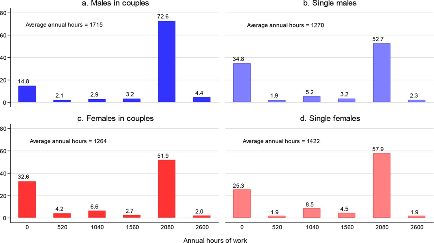
Distributions of discretised hours of work.
Source: Authors’ calculations based on the ILCS 2016 data.
Notes: The bar height measures the share (in %) of persons working the corresponding number of work hours annually. Sample sizes: 1,444 males from couples, 621 single males, 1,444 females from couples, 423 single females.
There are sizeable gender differences in the sample of couples. First, the females’ non-participation rate (approximately 1/3) is more than twice that of males (approximately 15%). Second, while almost 3/4 of males work full-time, only slightly more than half of females do so. In contrast, the gender differences in the sample of singles are reversed and are considerably smaller. First, non-participation is more prevalent among single males (1/3) than among single females (1/4). Second, more than half of both single males and females work full-time hours, with the women’s share exceeding the men’s by approximately five percentage points. As a consequence, males from couples participate more than single males, while the opposite holds for women; additionally, among the males from couples, there are relatively more individuals working full-time hours than there are among single men, while the opposite holds for women. All these couple-single and male-female differences are clearly reflected in the average number of annual hours of work (reported in Figure 1 as well).
4. Labour supply estimation results
4.1. Parameter estimates for couples
The estimates of the labour supply model parameters for couples are displayed in Table 2.[18] The deterministic part of utility is increasing in consumption as follows: the parameters of the variables involving consumption imply a positive marginal utility of consumption, and this holds for all values of consumption and for all male-female combinations of leisure hours observed in the data. Utility is increasing as well in each spouse’s leisure, and again this is true for all observed levels of consumption and leisure hours. We find evidence of a decreasing marginal utility of income and each spouse’s leisure hours, although in the case of male leisure hours, the result is not significant. The parameters of the interaction between consumption and leisure hours are not significant for either gender, suggesting no solid evidence that consumption and leisure are either substitutes or complements. Nevertheless, if anything, the positive signs of the estimates suggest that the relationship is closer to complementarity than to substitutability. On the other hand, there is significant evidence that the leisure hours of spouses are complements to one another.
Estimates of preference and opportunity parameters for couples.
| Parameter | Estimate | Std. err. | |
|---|---|---|---|
| Preferences | |||
| 0.464 | [0.214]* | ||
| −0.005 | [0.002]* | ||
| 4.606 | [2.858] | ||
| −0.115 | [0.167] | ||
| 10.769 | [2.506]*** | ||
| −0.434 | [0.149]** | ||
| 0.023 | [0.017] | ||
| 0.009 | [0.011] | ||
| 0.267 | [0.060]*** | ||
| −0.188 | [0.056]** | ||
| 0.002 | [0.001]** | ||
| 0.059 | [0.083] | ||
| 0.401 | [0.123]** | ||
| 0.641 | [0.228]** | ||
| −0.204 | [0.042]*** | ||
| 0.002 | [0.000]*** | ||
| 0.200 | [0.067]** | ||
| 0.194 | [0.109] | ||
| 0.959 | [0.231]*** | ||
| Male opportunity measure | |||
| 4.164 | [1.115]*** | ||
| −0.211 | [0.027]*** | ||
| 0.180 | [0.017]*** | ||
| Female opportunity measure | |||
| 3.203 | [0.716]*** | ||
| −0.167 | [0.019]*** | ||
| 0.136 | [0.012]*** | ||
| Male and female opportunity densities | |||
| 2.901 | [0.115]*** | ||
| 2.865 | [0.121]*** | ||
| Log-likelihood | −2,477.53 | ||
| No. of couples | 1,444 | ||
-
Source: Authors’ estimation using ILCS 2016 data.
-
Notes: Maximum simulated likelihood estimates with 50 simulations. */**/*** indicate statistical significance at the 10/5/1% level. 1[.] is an indicator variable that equals one if the condition in parentheses is true, and zero otherwise. C is measured in tens of thousands of HRK. LM and LF are measured in thousands of hours. Age and experience are measured in years.
The parameters of the interactions of leisure hours with observable characteristics point to a significant preference heterogeneity with respect to age, health conditions and parenting. For both spouses, the marginal utility of leisure is U-shaped with respect to age, being higher for younger and older people than for those in-between. Moreover, an additional hour of leisure is more preferred by people with health conditions that limit activity, especially if the limitation is severe. Finally, parenting more preschool children is associated with a higher marginal utility of leisure, but only for women. This result is in accordance with women’s behaviour and attitudes conforming to the rather firmly established tradition of considering child rearing as “women’s business”.
For both genders, there is a significant heterogeneity observed in the market opportunity measure: the job opportunities differ with respect to both age and work experience. Being younger and having more work experience expands one’s job opportunities. The negative impact of age might be due to employers’ preference for younger workers, conditional on work experience, a phenomenon that may be partly due to a type of discrimination and partly due to older worker’s relatively low readiness to adapt to the rapid technological changes characterising the modern economy. Concerning the positive effect of work experience, this is an intuitively expected result, given how employers value experience when hiring. The effects of both age and experience are stronger for men, perhaps because other factors affecting market opportunities might be more important for women. For example, whether a person has (or plans to have) children is likely more important for women’s market opportunities, especially given the recent unfortunate tendency of some employers to prefer childless female workers over those with small children. Finally, the parameters of the full-time peaks, which are meant to capture the intensity of full-time job offers for males and females compared to job offers with other work time regimes, are both positive and highly significant, indicating that for both males and females full-time jobs are offered significantly more frequently than other working time arrangements.
4.2. Parameter estimates for singles
The estimates for singles are given in Table 3. As in the case of couples, for singles of both genders, the marginal utilities of consumption and leisure are positive. This holds at any observed combination of values of the variables that consumption and leisure are interacted with (including themselves). For both men and women, we find significant evidence of diminishing marginal utilities of consumption and leisure, and unlike for males in couples, the result for single males is significant, though only marginally. Here, again, we do not find significant evidence that consumption and leisure are either substitutes or complements. However, we note that while for couples both estimates were positive (pointing to complementarity), here the insignificant estimate for females is negative (pointing to substitutability). Admittedly, it is difficult to speculate about the reasons for this sign reversal, but the estimates are insignificant anyway.
Estimates of preference and opportunity parameters for singles.
| Parameter | Males | Females | |||
|---|---|---|---|---|---|
| Estimate | Std. err. | Estimate | Std. err. | ||
| Preferences | |||||
| 0.404 | [0.177]* | 0.825 | [0.237]** | ||
| −0.006 | [0.002]** | −0.006 | [0.003]* | ||
| 12.797 | [3.809]** | 27.226 | [4.830]*** | ||
| −0.586 | [0.248]* | −1.365 | [0.300]*** | ||
| 0.007 | [0.019] | −0.024 | [0.026] | ||
| −0.157 | [0.045]** | −0.230 | [0.061]*** | ||
| 0.002 | [0.001]** | 0.002 | [0.001]** | ||
| 0.071 | [0.256] | ||||
| 0.776 | [0.165]*** | 0.366 | [0.203] | ||
| 1.413 | [0.395]*** | 0.561 | [0.553] | ||
| Opportunity measure | |||||
| 3.267 | [1.144]** | 4.567 | [1.275]*** | ||
| −0.229 | [0.030]*** | −0.261 | [0.038]*** | ||
| 0.202 | [0.020]*** | 0.174 | [0.028]*** | ||
| Opportunity density | |||||
| 2.718 | [0.183]*** | 2.614 | [0.215]*** | ||
| Log-likelihood | −550.02 | −394.81 | |||
| No. of individuals | 621 | 423 | |||
-
Source, Authors’ estimation using ILCS 2016 data.
-
Notes: Maximum simulated likelihood estimates with 50 simulations. */**/*** indicate statistical significance at the 10/5/1% level. 1[.] is an indicator variable that equals one if the condition in parentheses is true, and zero otherwise. C is measured in tens of thousands of HRK. LM and LF are measured in thousands of hours. Age and experience are measured in years.
The observed heterogeneity in the marginal utility of leisure is more pronounced for males, where there is significant heterogeneity with respect to age and health conditions. Since there are no single males with preschool children in the sample, the interaction between leisure and the number of preschool children is not included in the model for single males. Similar to males in couples, single males’ marginal utility of leisure is U-shaped with respect to age; it is higher for relatively young and old men. Single men with relatively bad health (especially when the condition is severe) prefer leisure more than the healthy ones, and the impact of health is stronger for single men than for men in couples. On the other hand, the marginal utility of leisure for women appears to systematically vary only with respect to age, where again a U-shaped pattern is observed. Moreover, single women’s preferences for leisure do not seem to depend on the presence of preschool children, although the estimate is only marginally short of significance at the 10% level. It might be that, being single mothers and, thus, single breadwinners, these women have preferences similar to those of men in couples, for which we also found that the number of preschool children does not seem to matter. Unlike for women and men in couples, health conditions do not significantly shape single women’s preferences. However, the estimates are positive, as expected. The estimate pertaining to health limitations falls marginally short of significance at the 10% level, while that pertaining to severe health limitations is not significant due to only a small fraction of single women having this health status (less than 2%).
The estimates of the parameters affecting job opportunities are very similar to those obtained for couples, showing that age is opportunity-reducing and work experience is opportunity-increasing for both men and women, with significant full-time peaks in the distribution of positive work hours.
4.3. In-sample and out-of-sample prediction performance
We now assess the in-sample and out-of-sample prediction performance of the model. If the model will be used for simulations of the effects of tax-benefit reforms, it should perform well in this regard.
We first assess the in-sample prediction performance by checking if the model is able to reproduce the observed discretised distribution of annual hours of work in the samples of couples and singles used for the estimation of the model. Precisely, we compare the shares of individuals observed to choose each of the discrete alternatives with the corresponding model-predicted choice probabilities. The fit is assessed for the marginal distribution of each gender, as well as for the joint male-female distribution. In addition, the fit is assessed with respect to household disposable income as well: the observed distribution is compared to the predicted.
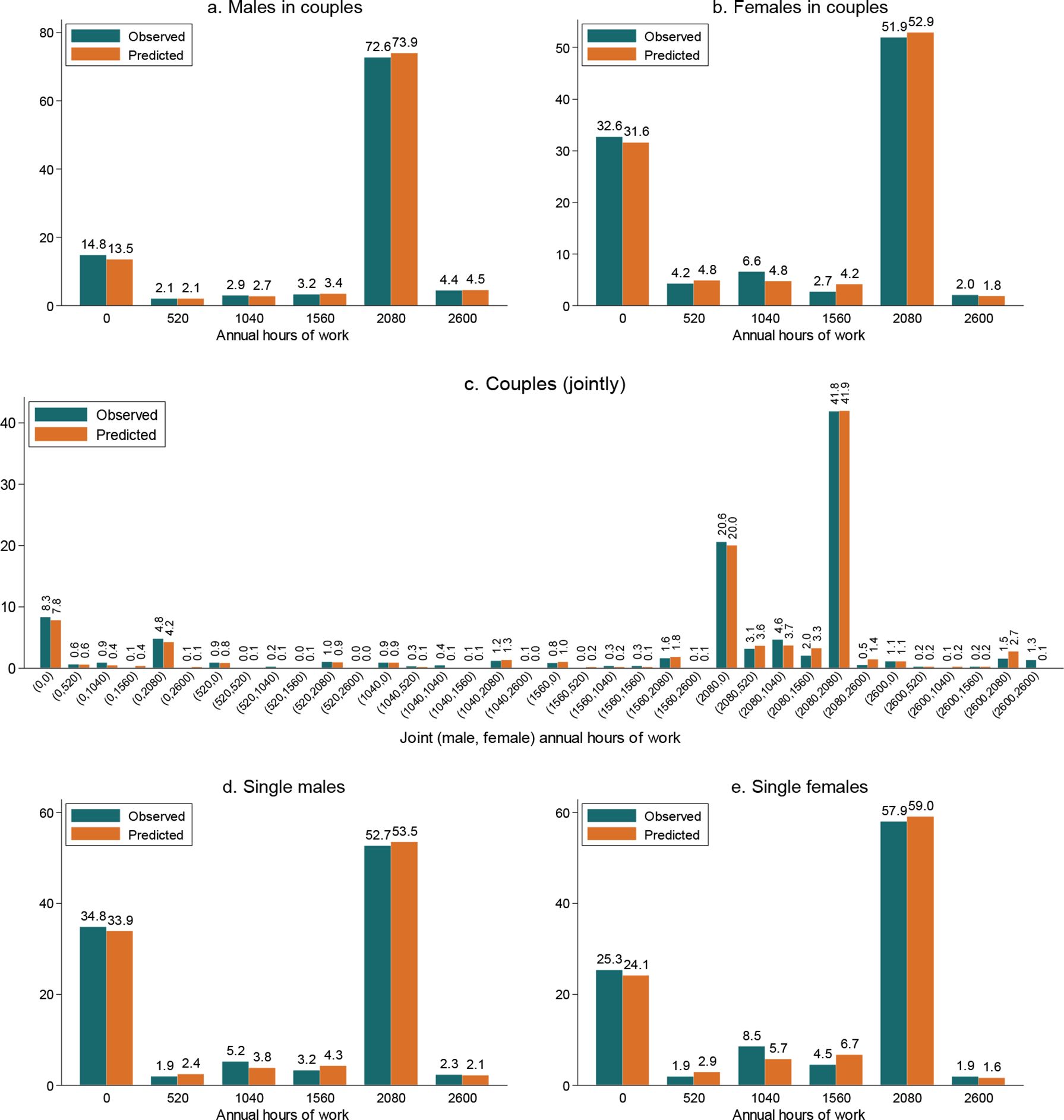
The comparisons of the observed and predicted distributions of work hours for males and females in couples are displayed in Figure 2. The fit for the marginal distributions appears to be very good for both males (panel a) and females (panel b). For both genders, the average predicted choice probability of non-participation is slightly smaller, ie, by approximately one percentage point, than the share of people observed not to participate. The opposite holds for the full-time hours (2080 hours). The fit is good for the remaining alternatives as well. It is almost perfect for men, with differences of at most 0.2 percentage points and is somewhat worse for women, but still reasonably good. A good fit for the marginal distributions does not, however, necessarily guarantee a good fit of the joint distribution. Thus, we check the fit for the latter as well. As shown on panel c, the predicted distribution is very well in line with the observed one, not only for the alternatives with relatively large masses but also for those scarcely represented in the sample.

In-sample prediction performance: observed and predicted distributions of hours of work.
Source: Authors’ calculations based on the ILCS 2016 data and the estimates of the labour supply model given in Table 2 (for males and females in couples) and Table 3 (for singles).
Notes: The height of each bar labelled “observed” measures the share of males (panel a), females (panel b) or couples (panel c) observed to work the corresponding number of hours annually in 2015. The annual work hours are the hours after discretisation of their actually observed distribution. The height of each bar labelled “predicted” measures the sample average of the probability to work the corresponding number of hours or, in the case of the joint male-female distribution, the corresponding male-female combination of hours. The probabilities are calculated using the parameters of the labour supply model and data for 2015.
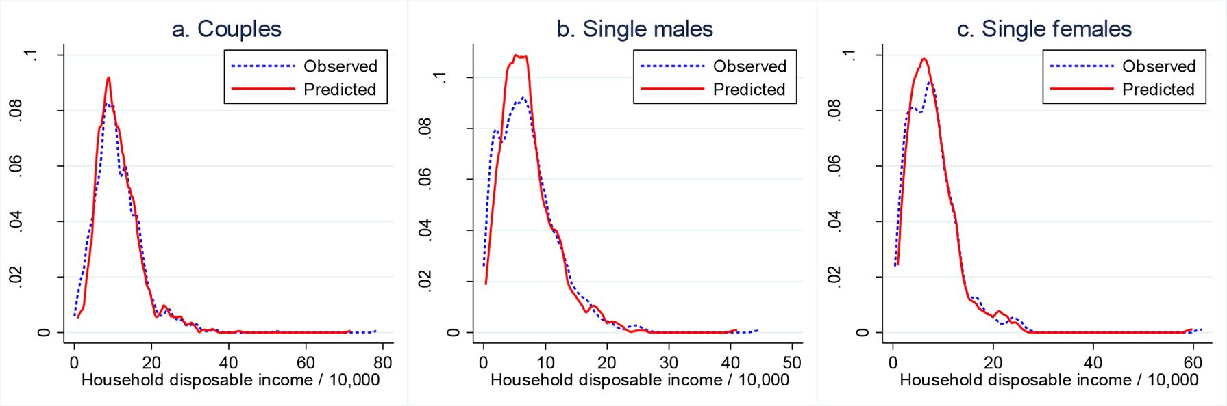
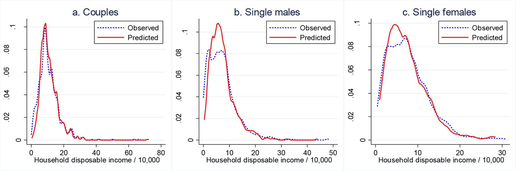
In Figure 3, we compare the observed distributions of total household disposable income compared to the predicted ones. This comparison also confirms the model’s good prediction performance. Although there are some differences between the observed and predicted densities, the two are aligned reasonably well, though not perfectly.

In-sample prediction performance: observed and predicted densities of total household disposable income.
Source: Authors’ calculations based on the ILCS 2016 data and the estimates of the labour supply model given in Table 2 (for males and females in couples) and Table 3 (for singles).
Notes: The densities are kernel estimates. The “observed” density refers to the density of total household disposable income actually observed in the 2015 data. The “predicted” density refers to the density of the expected total household disposable income, where the expectation is taken over the alternative-specific incomes, with the choice probabilities as weights. The choice probabilities are calculated using the parameters of the labour supply model and data for 2015.
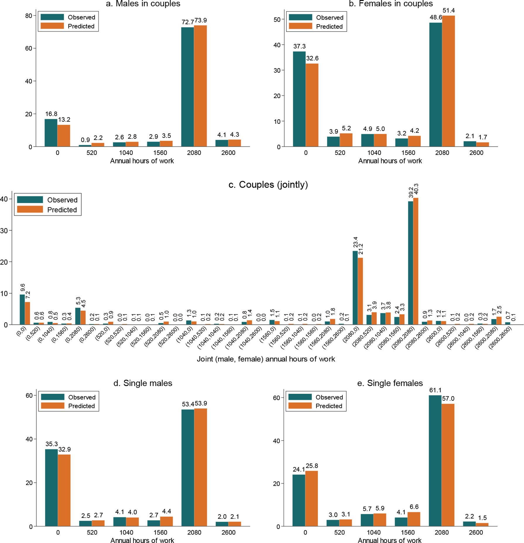
If the model’s parameters are truly structural, the model should also perform well in out-of-sample predictions. However, a good out-of-sample prediction performance is not guaranteed by a good in-sample prediction performance. Thus, we use the model to test the out-of-sample prediction performance. We take the parameters estimated for the data for the year 2015 (reported and discussed above) and the data for the year 2014 to assess how well the model can reproduce the distributions of hours of work and household disposable income for the latter year. The data source is the same, namely, the ILCS, and miCROmod is used to model the details of the tax-benefit system in 2014. As shown in Figure 4, the observed and predicted distributions of the hours of work are aligned in the 2014 data as well as they were in the 2015 data. This holds equally for the gender-specific marginal distributions (panels a and b) and the joint male-female distribution (panel c). The good out-of-sample prediction performance is corroborated through the comparison of the observed and predicted densities of household disposable income (Figure 5).

Out-of-sample prediction performance: observed and predicted distributions of hours of work.
Source: Authors’ calculations based on the ILCS 2015 data and the estimates of the labour supply model given in Table 2 (for males and females in couples) and Table 3 (for singles).
Notes: The height of each bar labelled “observed” measures the share of males (panel a), females (panel b) or couples (panel c) observed to work the corresponding number of hours annually in 2014. The annual work hours are the hours after discretisation of their actually observed distribution. The height of each bar labelled “predicted” measures the sample average of the probability to work the corresponding number of hours or, in the case of joint male-female distribution, the corresponding male-female combination of hours. The probabilities are calculated using the parameters of the labour supply model for 2015 and data for 2014.

Out-of-sample prediction performance: observed and predicted densities of total household disposable income.
Source: Authors’ calculations based on the ILCS 2015 data and the estimates of the labour supply model given in Table 2 (for males and females in couples) and Table 3 (for singles).
Notes: The model is estimated on the 2015 data, and the estimated parameters are used to predict the choice probabilities in the 2014 data. These probabilities are used in the calculation of the expected total disposable income for each household in the 2014 data. The density of this income is labelled “predicted”. The density labelled “observed” is the density of actually observed total household disposable income in the 2014 data.
A word of caution is in order here. A more credible assessment of the model’s out-of-sample performance would be to check if the model fits the data well from a year more distant from 2015 than 2014 is. Precisely, we would ideally use a year when the tax-benefit system and the distributions of hours of work and disposable income were more different from those in 2015. With respect to the tax-benefit system and the distributions of hours of work and disposable income, 2014 is very similar to 2015, thus, good out-of-sample performance is expected. This, however, makes the assessment of the out-of-sample prediction performance less credible. Unfortunately, only the data for 2015 (ILCS 2016) and 2014 (ILCS 2015) were available to us.
4.4. Elasticities of labour supply
We compute the following two elasticities of labour supply: the elasticity of participation and the elasticity of work hours. More precisely, the elasticity of participation is the elasticity of the probability of participation (ie, the probability of working non-zero hours), as predicted by the model. It is defined as the proportional change in the probability of participation induced by a proportional increase in the gross wage rate, divided by that proportional increase in the gross wage rate. The elasticity of work hours is the elasticity of the expected work hours, where the expectation is taken over the discrete alternatives (36 for people from couples, 6 for singles), with the model-predicted choice probabilities as weights.
Both elasticities are the so-called “aggregate” elasticities. Precisely, in the case of elasticity of participation, the average individual probability of participation is first obtained by averaging over the sample. The aggregate elasticity of the probability of participation is then calculated as the proportional change in the average probability of participation divided by the proportional rise in the gross wage. Similarly, in the case of elasticity of work hours, the average individual expected work hours are calculated by averaging over the sample. The aggregate elasticity of work hours is then obtained as the proportional change in the average individual expected hours divided by the proportional increase in the gross wage.[19]
For the calculation of both elasticities, a 10% gross wage increase is assumed. For males and females in couples, the elasticities are calculated with respect to both their own gross wage (own elasticity) and their partner’s/spouse’s gross wage (cross elasticity).[20] The elasticities are displayed in Table 4 for couples and in Table 5 for singles. In the first row of each table (labelled “All”) are the elasticities computed for the whole sample, without conditioning on any attribute apart from gender and relationship status. The remaining elasticities pertain to narrower samples, defined according to such attributes as the household’s income quintile, age, education, having a preschool child and the number of minor children.
Elasticity of the labour supply for couples.
| Elasticity of the probability of participation | Elasticity of the expected work hours | |||||||
|---|---|---|---|---|---|---|---|---|
| Males | Females | Males | Females | |||||
| Own elasticity | Cross elasticity | Own elasticity | Cross elasticity | Own elasticity | Cross elasticity | Own elasticity | Cross elasticity | |
| All | 0.179 | −0.010 | 0.325 | −0.030 | 0.232 | −0.017 | 0.423 | −0.046 |
| Income quintile group | ||||||||
| first | 0.498 | 0.035 | 0.677 | 0.046 | 0.593 | 0.037 | 0.823 | 0.043 |
| second | 0.212 | −0.005 | 0.442 | −0.026 | 0.276 | −0.008 | 0.569 | −0.035 |
| third | 0.126 | −0.013 | 0.336 | −0.017 | 0.179 | −0.016 | 0.454 | −0.027 |
| fourth | 0.102 | −0.025 | 0.238 | −0.051 | 0.148 | −0.036 | 0.328 | −0.071 |
| fifth | 0.072 | −0.026 | 0.166 | −0.056 | 0.109 | −0.039 | 0.237 | −0.080 |
| Age | ||||||||
| 30 or less | 0.135 | 0.003 | 0.484 | −0.015 | 0.218 | 0.001 | 0.699 | −0.049 |
| 31–50 | 0.144 | −0.007 | 0.311 | −0.033 | 0.195 | −0.014 | 0.408 | −0.048 |
| 50 or more | 0.285 | −0.020 | 0.314 | −0.025 | 0.341 | −0.029 | 0.382 | −0.036 |
| Education | ||||||||
| Low | 0.344 | 0.020 | 0.567 | 0.012 | 0.421 | 0.023 | 0.690 | 0.002 |
| Middle | 0.180 | −0.009 | 0.339 | −0.034 | 0.237 | −0.016 | 0.446 | −0.050 |
| High | 0.108 | −0.025 | 0.226 | −0.034 | 0.145 | −0.036 | 0.306 | −0.053 |
| Preschool children (age 0–6) | ||||||||
| No | 0.182 | −0.013 | 0.292 | −0.033 | 0.233 | −0.021 | 0.377 | −0.046 |
| Yes | 0.171 | −0.002 | 0.425 | −0.021 | 0.231 | −0.006 | 0.575 | −0.047 |
| Number of children (age 0–17) | ||||||||
| No | 0.226 | −0.021 | 0.302 | −0.036 | 0.280 | −0.030 | 0.382 | −0.050 |
| 1 or 2 | 0.149 | −0.008 | 0.318 | −0.030 | 0.200 | −0.015 | 0.420 | −0.048 |
| 3 or more | 0.224 | 0.005 | 0.444 | −0.013 | 0.287 | 0.001 | 0.578 | −0.025 |
-
Source: Authors’ calculationsbased on the estimates of the labour supply model from Table 2 and the ILCS2016 data.
-
Notes: For definitions of the elasticities, see Section 4.4. The elasticities are calculated assuming a 10% increase in the gross wage, either the individual’s own (for own elasticities) or that of the partner (for cross elasticities). Income refers to the expected household disposable income equivalised using the modified OECD equivalence scale; the expectation is taken over the 36 alternatives, with the estimated choice probabilities as weights.
Elasticity of the labour supply for singles.
| Elasticity of the probability of participation | Elasticity of the expected work hours | |||
|---|---|---|---|---|
| Males | Females | Males | Females | |
| All | 0.266 | 0.276 | 0.305 | 0.346 |
| Income quintile | ||||
| first | 0.598 | 0.695 | 0.663 | 0.822 |
| second | 0.352 | 0.364 | 0.405 | 0.463 |
| third | 0.242 | 0.319 | 0.289 | 0.403 |
| fourth | 0.216 | 0.174 | 0.252 | 0.241 |
| fifth | 0.150 | 0.089 | 0.170 | 0.132 |
| Age | ||||
| 30 or less | 0.294 | 0.337 | 0.368 | 0.517 |
| 31–50 | 0.248 | 0.263 | 0.284 | 0.332 |
| 50 or more | 0.291 | 0.272 | 0.317 | 0.304 |
| Education | ||||
| Low | 0.316 | 0.487 | 0.357 | 0.557 |
| Middle | 0.251 | 0.307 | 0.293 | 0.388 |
| High | 0.282 | 0.200 | 0.304 | 0.260 |
| Preschool children (age 0–6) | ||||
| No | 0.266 | 0.272 | 0.305 | 0.342 |
| Yes | – | 0.326 | – | 0.418 |
| Number of children (age 0–17) | ||||
| No | 0.268 | 0.267 | 0.309 | 0.336 |
| 1 or 2 | 0.189 | 0.298 | 0.051 | 0.371 |
| 3 or more | – | 0.389 | – | 0.480 |
-
Source: Authors’ calculations based on the estimates of the labour supply model from Table 3 and the ILCS 2016 data.
-
Notes: For definitions of the elasticities, see Section 4.4. The elasticities are calculated assuming a 10% increase in gross wage, either own (for own elasticities) or the partner’s (for cross elasticities). Income refers to the expected household disposable income equivalised using the modified OECD equivalence scale; the expectation is taken over the six alternatives, with the estimated choice probabilities as weights. There are no single males with children aged 0–6 or with three or more children.
All the own elasticities are positive, as expected, indicating that higher wages, other things equal, make work more attractive, thus increasing both participation and work hours. In contrast, most cross elasticities are negative but very small: a higher spouse’s/partner’s wage acts as a disincentive to work (more), but the disincentive effect is practically negligible, especially for males. For that reason, from here on, we focus exclusively on the elasticities with respect to the individual’s own wage. In couples, females’ elasticities are, in general, considerably larger than males’, which is a consequence of generally lower participation rates and average work hours for females. Similarly, the elasticities for single females tend to be higher than those for single males, but the tendency is not as strong as in the case of couples. For example, single females’ elasticities are higher than those of single males in the bottom three income quintiles, in age groups younger than 50, in groups with at most a middle educational level and irrespective of the number of minor children; in the remaining groups, the opposite holds. The elasticities for single males are mostly larger than for males from couples, as the former have a lower labour supply, in terms of both participation and average annual hours. The opposite holds for females, as females from couples participate less and work fewer hours on average than single females.
There is quite some heterogeneity in the elasticities by the income quintile, age, education, whether one has a preschool child, and the number of minor children. The elasticities are highest in the first income quintile, declining monotonically towards the fifth quintile. This pattern, which is commonly observed in the literature, is due primarily to the fact that the participation rate and the average number of work hours are lowest at the bottom of the income distribution. Indeed, given the high importance, on average, of labour income for total family income, the low labour supply is a major reason for being at the bottom of the income distribution. In most cases, the same monotonic pattern is observed with respect to education: elasticities are declining with the level of education. In regard to age, the elasticities for the youngest (30 or less) and oldest (50 or more) tend to be higher than for those in-between, mainly due to higher labour supply of the latter. Females’ elasticities are much more affected than those of males by whether one parents a preschool child and how many minor children one has: those with preschool children and those with more minor children have higher elasticities.
5. Making work pay in Croatia
5.1. Labour market situation
In terms of labour market conditions, Croatia is among the worst performers within the EU. The inactivity rate for the population aged 20–64 is as high as 28%, which is well above the EU-28 average of 23% and the third highest in the EU. Inactivity is especially high for females (33%) and is 10 percentage points higher than for males.[21] In addition to high inactivity, as much as 16% of the active population is unemployed, which is seven percentage points above the EU-28 average and is the third highest; little difference is found between males and females. Long-term unemployment is another problem: the share of long-term unemployment is two thirds (again the third highest) compared to the EU-28 average of approximately one half.
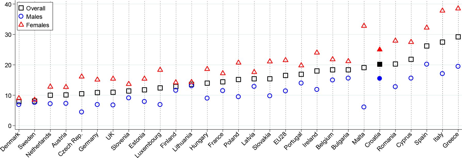
Although the above figures are telling enough about the issues of the Croatian labour market, we also consider a labour market aggregate that better corresponds to our classification of flexible people into participants (h>0) and non-participants (h=0). Recall from Section three that, besides the employed and the unemployed, the flexible persons include all inactive persons who are not in education or training, are not retired and are not unable to work. Then, the employed are considered to be participating, and the rest are considered to be not participating. In a recent paper, Nestić and Tomić (2018) extend the NEET (not in employment, education or training) concept beyond the youth population. In particular, they consider the whole population aged 20–64, and define the extended NEETs[22] as those not in employment, education, training, retirement or disability. Thus, conceptually this aggregate corresponds largely, though not perfectly, to our non-participating flexibles.[23] As shown in Figure 6, Croatia has one of the highest extended-NEET rates in the EU; only five countries have a higher rate.

Population aged 20–64 not in employment, education, training, disability or retirement.
Source: Authors’ calculations based on Eurostat data on the unemployment rates, the inactivity rates and the structure of inactivity by the main reason.
This unfavourable labour market situation has arisen due partly to the economic crisis that hit Croatia particularly severely. However, the underlying reasons for the high inactivity and unemployment seem to be mainly structural, rather than cyclical, and Croatia is, in that respect, similar to other south and south-east European countries. Since the adverse labour market impact of the economic downturn was stronger (and the subsequent recovery weaker) than in other EU countries, it also seems that the structural weaknesses amplified the cyclical factors.
5.2. In-work benefits as make-work-pay instruments
As many theoretical and empirical contributions suggest, one structural factor that may be at play is the design of the tax-benefit system, insofar as it impacts work incentives.[24] Various redistributive instruments – both taxes and benefits – and their disincentive effects with respect to the labour supply have been particularly emphasised in both scholarly work and policy circles. Policy makers across countries have realised that redistribution towards the needy, in the form of income support programmes for those out of work, can create significant work disincentives for the beneficiaries or their family members. In other words, pursuing equity objectives may have not only direct costs (social protection expenditures) but also indirect, efficiency costs (lower labour supply). Thus, some countries decided to try to reconcile the equity and efficiency objectives by implementing social protection instruments that “make work pay” (for a review, see Matsaganis and Figari, 2016).
One of these types of instruments are the so-called in-work benefits (henceforth, IWBs).[25] The idea is to incentivise the needy to find employment by providing higher transfers to those who work but earn a low income than to those who do not work (although they are able to work). Unlike the traditional social benefits that are granted to people out of work, IWBs are conditional on employment, which is their most important distinguishing feature. An IWB is usually designed to have the following features: (i) a phase-in region, starting at some relatively low number of work hours (or some low amount of income earned), in which the amount of the benefit is increasing with work hours (or income), implying a negative marginal effective tax rate; (ii) a maximum amount of benefit paid to those who reach a certain number of hours (amount of income); (iii) a phase-out region in which the amount of the benefit is falling with the work hours (or income), up to a maximum number of work hours (amount of income), where the benefit drops to zero. In an optimal taxation framework, Saez (2002) has shown that if people choose their labour supply on both the extensive margin (whether to work or not) and the intensive margin (how much to work conditional on working), and if the labour supply responses of people from low-income families are more concentrated at the extensive than at the intensive margin, then social benefits with the above three features are likely to be optimal (that is, social welfare-maximising).
Whether an IWB will have the intended effects of making it more attractive for people to work and receive higher transfers than to stay out of work and receive lower transfers, depends on its design. A design feature that has proven crucial so far concerns the level at which the income test of eligibility is done. In that respect, the following two types of IWBs are distinguished: (a) family-based and (b) individual-based. The pioneering IWBs, introduced in the US and the UK in the early 1970s, known today as the Earned Income Tax Credit (EITC) and the Working Tax Credit (WTC), respectively, are family-based. The income test is done at the family level, by adding up the market incomes of all family members and comparing it to a threshold. Family based IWBs have the quality of being well targeted towards needy families, rather than to low-income individuals from relatively well-off families. However, this, in principle, comes at the price of significant work disincentives (high participation tax rate) for potential second earners if their potential earnings (to be realised upon eventual employment) are high enough to make the family ineligible for the IWB, according to the family income test. For that reason, some countries (for example, the Netherlands, Belgium, Sweden and Finland) decided to implement individual-based IWBs, where the income test is done at the level of the individual. The work disincentives for potential second earners are avoided in this way, but again, there is a price to be paid: individual-based IWBs may not be well targeted, as a beneficiary can be a low-earning person from a relatively well-off family. Thus, in general, there is a trade-off between how well targeted an IWB is and how much of a work incentive it provides for potential second earners.[26]
A growing empirical literature using quasi-experimental identification methods finds, in general, that IWBs increase the labour supply of the beneficiaries at the extensive margin, thus, raising their families’ disposable income. On the other hand, there is little evidence of substantial labour supply responses at the intensive margin. Most quasi-experimental evaluations of the labour supply effects of the EITC in the US show that it has a significant positive impact on employment (for example, Eissa and Liebman, 1996; Eissa and Hoynes, 2004; Eissa and Hoynes, 2006; Meyer and Rosenbaum, 2001; Chetty et al., 2013).[27] The results for other countries – such as the UK (Blundell et al., 2005; Leigh, 2007; Francesconi and van der Klaauw, 2007), Canada (Card and Hyslop, 2005; Milligan and Stabile, 2007), Sweden (Laun, 2017) and the Netherlands (Bettendorf et al., 2014) – are similar in nature, if not in magnitude, all showing positive employment impacts of IWBs.[28]
Another growing strand of literature, where the present paper belongs to, evaluates the labour supply effects of IWBs ex-ante, using behavioural microsimulations. These studies, mostly done for European countries, often focus on the dependence of the labour supply effects of IWBs on their design, especially with respect to the family/individual-based distinction. An exemplary study is that of Bargain and Orsini (2006), who simulate the effects of two IWBs – one family-based, one individual-based – on social inclusion (employment) and poverty in Finland, France and Germany. They conclude, as the theory predicts, that the family-based IWB is more suitable for poverty reduction, while the individual-based IWS is better for increasing employment. Thus, the choice between the two crucially depends on the policy maker’s objectives. Broadly similar conclusions are reached by Vandelannoote and Verbist (2016), based on simulations for Belgium. Perhaps of greater importance for the present paper are the analyses for south and southeast European countries. Figari (2010) simulates family- and individual-based IWBs for Greece, Italy, Portugal and Spain. He finds that the expected trade-off between the redistributive and incentive effects is present but is rather weak if the employment rate of secondary earners (mostly women) is low. This points to the importance of the current labour market circumstances on the effects of IWBs. Focusing exclusively on married women and single mothers in Italy, Figari (2015) finds that both individual- and family-based IWB schemes can increase female participation and that it is possible to achieve more redistribution and efficiency at the same time. In another Italian study, Luca et al. (2014) show that the trade-off between efficiency and redistribution can be mitigated to some extent through a double-earner premium, with the remaining trade-off depending on the size of the premium. Ayala and Paniagua (2018) simulations suggest that IWBs would increase female participation in Spain as well. In the Western Balkan context, the studies of Mojsoska Blazevski et al. (2015) and Ranđelović et al. (2013) indicate potentially favourable employment effects of IWBs in Macedonia and Serbia, respectively. Both studies show that individual-based IWBs are more effective in incentivising potential second earners.
5.3. Basic features of the Croatian tax-benefit system
We briefly describe the Croatian system of direct taxes and cash social benefits in 2015, focusing on the most important instruments.[29] All the amounts that we mention here are monthly amounts. For comparison, the average gross monthly employment income, calculated from the ILCS data for 2015, is approximately HRK 6,800. Employer and employee social insurance contributions (SIC) amount to 17.2% and 20% of gross earnings. The personal income tax (PIT) base for an employee equals gross earnings minus employee SIC, basic personal allowance (HRK 2,600) and allowances for dependent members (HRK 1,300; 1,820; 2,600 for the first, the second, the third child; and HRK 1,300 for adult dependants). The PIT base is divided into three parts, taxed by the marginal rates of 12% (HRK 0–2,200), 25% (HRK 2,200–13,200) and 40% (beyond HRK 13,200). Cities and municipalities impose a surtax, whose base is the PIT amount, and the rates are 0–10% in municipalities and 0–18% in cities.
A social insurance system provides replacement incomes during periods of unemployment, sickness and parental leave. The unemployment benefit lasts between 3 and 15 months, depending on the time spent in employment before the job loss. During the first three months of unemployment, the benefit amounts to 70% of the net monthly earnings, while in the remaining period, this amount drops to 35% of the net monthly earnings. The maximum benefit amount equals 70% of the national average net monthly wage for the first three months and 35% of the national average net monthly wage for the remaining period.[30]
Two most important social benefits are the child benefit and the guaranteed minimum benefit. The child benefit is an income-tested benefit for households with children aged up to 15, or up to 19 if in secondary education. The net monthly household income per member may not be higher than HRK 1,663, and the benefit amount per child equals HRK 300, 250 or 200, depending on the income. There is also a supplement of HRK 500 (1000) for households with three (four or more) children, which was introduced as a pronatalist policy measure. The guaranteed minimum benefit is an asset- and income-tested benefit scheme for households with incomes below the “minimum subsistence amount”. The benefit amount equals the minimum subsistence amount minus the average net household income in the preceding 3 months. The minimum subsistence amounts for some typical households are as follows: HRK 800 for a single person; HRK 960 for a couple; HRK 1,600 for a couple with two children; HRK 1,660 for a lone parent with two children. In addition, the guaranteed minimum benefit recipients are eligible to receive compensation for electricity costs of HRK 200 per month, as well as compensation for housing costs, which are provided by cities and municipalities, with the ceiling amount set to 50% of the guaranteed minimum benefit amount.
5.4. The simulated in-work benefits
We simulate the effects of two in-work benefits. One is inspired by the Working Tax Credit in the United Kingdom (hereafter: WTC), and the other is inspired by the Employee Tax Credit in Slovakia (hereafter: ETC). EUROMOD (Sutherland and Figari, 2013) is used to “export” the policies from the UK and Slovakian tax-benefit systems and “import” them into the 2015 Croatian tax-benefit system, as modelled in miCROmodA. We do not import them in the exact form in which they exist in their home countries, however. While preserving the basic mechanism of the original policies, we simplify and adapt the original WTC and ETC.[31] We do these amendments for the sake of comparability between the WTC and ETC and to better fit the Croatian context. For example, some elements, such as the eligibility rules and definitions of the relevant income concepts, are aligned among the two benefits. No other changes to the Croatian tax-benefit system are introduced besides implementing the WTC or ETC, and both are excluded from the income used for income-testing the child benefit and the guaranteed minimum benefit.
The eligibility rules, income tests and benefit formulas for WTC and ETC are as follows:
Eligibility: Every person aged 18–65 who worked at least 520 hours in a given year is eligible. It does not matter how the minimum required hours are distributed over the year, eg, one may work 40 hours a week for three months, or 20 hours a week for six months, in continuity or with interruptions. It only matters whether a person worked at least 520 hours during the year.
Income test: Both benefits are income tested. The test income comprises the sum of the post-tax original and replacement incomes. In the case of ETC, only the income of the eligible person is taken into account, irrespective of whether the person is single or married. In contrast, the WTC also considers the income of the spouse if the person is married.
Benefit formula: The benefit amount (B) is given by the following formula:
| B=max{0, M – max[0, r ∙ (I – T)]} | (11) |
where M is the maximum benefit amount, I is the test income, T is the income threshold, and r is the benefit withdrawal rate.
Table 6 shows the parameters for the two benefits. For the WTC, the maximum benefit amount is the sum of the following four components: (a) Basic component – for all eligible workers, (b) Lone parent component – for lone parents, (c) Couple component – for persons who have partners, and (d) 1560 hours component – for persons who have worked at least 1560 hours per year, which is the equivalent of 9 months of work at a full-time job. In the case of ETC, all eligible workers are entitled to the same maximum benefit amount. Note that the maximum benefit amount is much larger in the WTC, but the withdrawal rate is also higher than in the ETC.
Parameters of WTC and ETC.
| WTC | ETC | |
|---|---|---|
| Maximum benefit amount, M | (a)+(b)+(c)+(d) | 3,623 |
| (a) Basic element | 6,735 | – |
| (b) Lone parent element | 6,907 | – |
| (c) Couple element | 6,907 | – |
| (d) 1560 hours element | 2,784 | – |
| Income threshold, T | 22,060 | 36,360 |
| Withdrawal rate, r | 0.41 | 0.19 |
-
Notes: All monetary parameters are expressed in HRK. These values of parameters ensure that the total amount of each benefit given to the sample couples is HRK 300 million in a framework without behavioural effects.
To illustrate the functioning of the two in-work benefits, we use examples with two hypothetical couples. An “actor” is a hypothetical non-employed person who considers what to do regarding his or her activity in the next 12 months and has two options in this “pre-decision situation”.[32] One option is to remain non-employed for the whole considered period. Alternatively, he or she can become employed for a certain number of months, with certain work hours per week and a certain monthly gross wage. We have two couples, A and B, in which the actors are spouses A2 and B2, respectively. In couple A, the other spouse, A1, is non-employed. In couple B, the spouse B1 is full-time employed (12 months during the year, 40 hours per week), earning 50% of the average monthly gross wage (AGW).
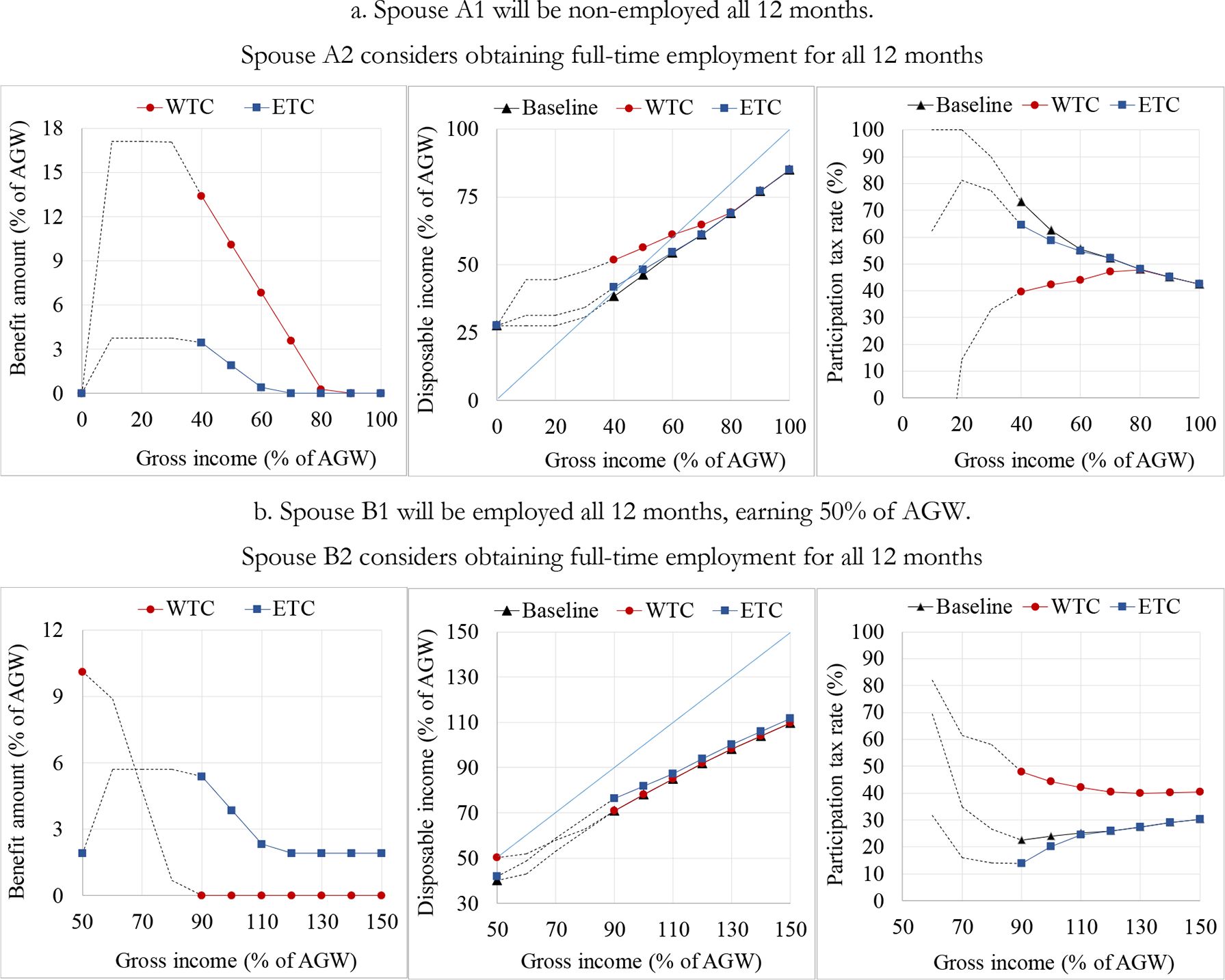
Figure 7 depicts the situations for couple A (panel a) and couple B (panel b). Spouses A2 and B2 consider whether to remain non-employed for the whole year, or to get a full-time job (40 hours per week) for the whole year. If they choose non-employment, the annual gross wage of A2 and B2 is zero. Otherwise, A2 and B2 can earn a monthly gross wage in the range from 40% to 100% of the AGW. The panels in Figure 7 show the benefit amount at the household level (left graph), the household disposable income (middle graph), and the participation tax rate faced by the actor (right graph), with each plotted against the household’s total gross employment income.
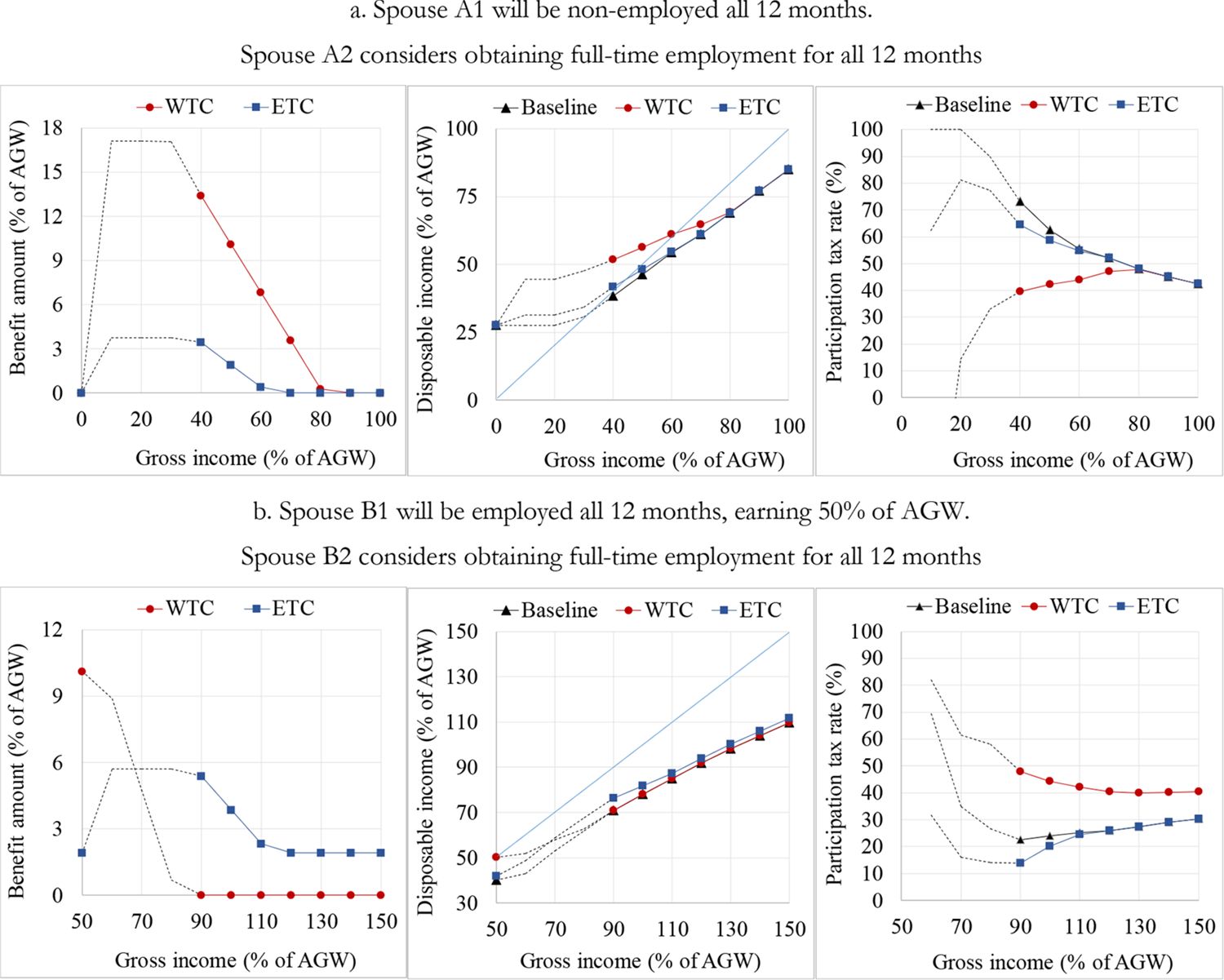
Illustration of the WTC and ETC with two hypothetical couples. a. Spouse A1 will be non-employed all 12 months. Spouse A2 considers obtaining full-time employment for all 12 months b. Spouse B1 will be employed all 12 months, earning 50% of AGW. Spouse B2 considers obtaining full-time employment for all 12 months
Notes: Gross income is the sum of the gross employment incomes of both spouses. The participation tax rate is one minus the change in disposable income taking place upon the transition from non-employment to employment, expressed as a share of gross income that would be earned in the case of employment. In panel a., the benefit amount and disposable income at a gross income of zero are identical for the WTC and ETC scenarios; therefore, the markers overlap, i.e., the one showing the WTC scenario is hidden. In Croatia in 2015, the minimum gross wage for full-time employment was approximately 38% of the average gross wage. Therefore, the actors A2 and B2 cannot be legally employed at a gross wage below the minimum wage. Accordingly, we show the results for gross wages beyond 38% of the AGW (represented by full lines and markers on the graphs). However, for the sake of illustration, the points below 38% of the AGW are also shown (represented by dotted lines on the graphs).
Source: Authors’ simulations using miCROmod.
Both spouses of couple A are non-employed in the pre-decision situation. If spouse A2 decides to remain non-employed, the benefit amount is zero for both WTC and ETC. If A2 becomes employed, the WTC provides much more generous support than the ETC (at least for gross wages of up to 80% of the AWG). For example, if A2 becomes employed at a gross wage of 40% of the AGW, the amount of the WTC is 13.4% of the AGW, compared to only 3.5% of the AGW in the case of the ETC. Both benefits provide incentive for participation, as both decrease the participation tax rate, but the WTC is much more effective than the ETC in this respect.
Quite a different picture is revealed for couple B. Because spouse B1 is already employed in B2’s pre-decision situation, the couple is receiving the WTC. If actor B2 becomes employed, the amount of the WTC falls due to the income test, which takes into account the couple’s total income. Even if B2 becomes employed at a low gross wage, for example, 40% of the AGW, the benefit amount falls to zero. This mechanism reduces incentives for participation by increasing the participation tax rate, which is substantially higher than in the baseline scenario. In contrast, in the case of the ETC, the benefit amount of a household increases if B2 obtains a job, and this increase occurs because the income test considers the incomes of the two spouses independently. The ETC decreases the participation tax rate if B2 becomes employed at a low gross wage, ie, up to 60% of the AGW.
5.5. Simulation results
The Baseline scenario simulates the actual tax-benefit system in 2015. Two counterfactual scenarios are created as follows: the WTC reform (ETC reform) scenario implements the WTC (ETC) into the tax-benefit system. We first simulate the effects on the labour supply, and then, taking the behavioural responses into account, we simulate the effects on the state budget, poverty and inequality. Simulations are performed for couples only, and the sample is the same as that for which the labour supply model for couples is estimated.
The two in-work benefits have different effects on the labour supply (Table 7). The WTC decreases the average probability of being employed at 2080 and 2600 hours for both males and females. In other words, individuals are more likely to choose less time intensive employment or to become non-employed. The probability of non-participation for males increases by 0.37 percentage points. For females, the increase is approximately twice as large, 0.79 percentage points. In contrast, the ETC decreases the probability of non-participation for both males and females by 0.35 and 1.17 percentage points, respectively. It also slightly decreases the probability of engagement in over-time work (2600 hours).
Aggregate effects of the WTC and ETC on the labour supply.
| Annual hours of work | ||||||
|---|---|---|---|---|---|---|
| 0 | 520 | 1040 | 1560 | 2080 | 2600 | |
| Males | ||||||
| a. Baseline | 13.36 | 2.04 | 2.63 | 3.39 | 74.09 | 4.49 |
| b. WTC reform | 13.74 | 2.18 | 2.79 | 3.52 | 73.42 | 4.35 |
| c. ETC reform | 13.02 | 2.08 | 2.80 | 3.50 | 74.16 | 4.45 |
| WTC reform vs. baseline (b – a) | 0.37 | 0.14 | 0.15 | 0.14 | −0.66 | −0.14 |
| ETC reform vs. baseline (c – a) | −0.35 | 0.04 | 0.16 | 0.11 | 0.07 | −0.04 |
| Females | ||||||
| d. Baseline | 30.60 | 5.34 | 5.01 | 4.24 | 53.00 | 1.81 |
| e. WTC reform | 31.39 | 5.40 | 4.99 | 4.23 | 52.23 | 1.76 |
| f. ETC reform | 29.43 | 5.39 | 5.26 | 4.43 | 53.71 | 1.79 |
| WTC reform vs. baseline (e – d) | 0.79 | 0.06 | −0.02 | −0.01 | −0.77 | −0.05 |
| ETC reform vs. baseline (f – d) | −1.17 | 0.05 | 0.25 | 0.19 | 0.71 | −0.03 |
-
Source: Authors’ simulations using miCROmod.
-
Notes: Each figure represents the probability of working a certain number of hours (0, 520, 1040, 1560, 2080 or 2600) in a certain scenario (baseline, WTC reform or ETC reform).
The labour supply effects reported in Table 7 are aggregate effects, pertaining to the entire sample of couples. The aggregate effects may, however, come as a net outcome of heterogeneous effects across different groups. We are particularly interested in the participation effects for males and females depending on the employment status of their spouses. Thus, for each gender, we compute the change in the average participation probability with the WTC and ETC reforms for those whose spouse is employed and for those whose spouse is not employed. As discussed before, the employment status of one’s spouse is likely to matter for one’s work incentives, and the importance of the spouse’s employment status is likely to depend on the type of in-work benefit (ie, whether it is individual- or family-based).
The results are shown in the upper part of Table 8. In the first row, we report the aggregate effect; these figures are equal to those reported in the first column of Table 7 (ie, for zero hours), multiplied by −one for convenience, so that they represent changes in the probability of participation, rather than non-participation. There are notable differences between the effects for persons whose spouses work and those whose spouses do not work. This is especially so in the case of the WTC, where one effect is positive and the other is negative. Precisely, upon the introduction of the WTC, the participation probability raises for males whose spouses do not work, and declines for those whose spouses work. The same holds for females, yet with notably stronger effects since the introduction of the WTC presumably leads to a greater income effect among females. For both genders, the negative aggregate effect is driven by the negative effect – decline in incentives for participation – for persons whose spouses work. In contrast, the ETC increases the participation probability for both genders irrespective of whether their spouses do or do not work, with an expectedly larger increase for those with non-working spouses. In summary, while the ETC improves the incentives for work independent of the spouse’s employment status, the WTC does so only if the spouse is not employed.
The effects of the WTC and ETC on the probability of participation for males and females depending on the employment status of their spouses.
| WTC reform vs. baseline | ETC reform vs. baseline | |||
|---|---|---|---|---|
| Males | Females | Males | Females | |
| Aggregate effect | −0.37 | −0.79 | 0.35 | 1.17 |
| a. Type-specific effect on the probability of participation | ||||
| Spouse not employed | 0.38 | 1.63 | 0.51 | 1.38 |
| Spouse employed | −0.74 | −1.21 | 0.27 | 1.14 |
| b. Contribution to the aggregate effect | ||||
| Spouse not employed | 0.13 | 0.24 | 0.17 | 0.20 |
| Spouse employed | −0.50 | −1.03 | 0.18 | 0.97 |
-
Source: Authors’ simulations using miCROmod.
-
Notes: Each figure represents the change (expressed in percentage points) in the probability of participation upon the introduction of the WTC or ETC. The aggregate effect is equal to the effect on the probability of non-participation (zero work hours) reported in the first column of Table 7, multiplied by –1; thus, it measures the change in the probability of participation (rather than non-participation) upon the introduction of the WTC or ETC. Panel (a) displays the changes in the participation probability for males and females depending on whether their spouses are employed or not. In panel (b), the aggregate effect is decomposed into the respective contributions of the two types: the aggregate effect equals the sum of the two contributions. Each contribution is calculated as the product of a type-specific effect from panel (a) and the share of that type in all males or females.
These results are in line with the structure of work incentives incorporated into the WTC, as we explained in the example with the hypothetical couple B (see Section 5.4), where only one partner participates at the time the other is considering whether or not to obtain a job. We saw that when one partner is already working, the other partner’s incentive to participate diminishes when the WTC is introduced and improves when the ETC is introduced. Moreover, note that for females whose spouse is not employed, the WTC increases the probability of participation more than the ETC does. This could also have been predicted based on differences in the structures of incentives to participate between the WTC and ETC for a couple where neither spouse works and one is considering whether to obtain employment. As we saw in the example with the hypothetical couple A, the higher generosity of the WTC makes it substantially more effective than the ETC in improving incentives for participation (up to a gross wage of 80% of the AWG). For males whose spouse is not employed, however, the ETC brings a larger increase in the participation probability. Nevertheless, the differences between the effects of the WTC and ETC are quite small both for males and females whose spouses do not work; thus, we should perhaps not draw any firm conclusions from these results.
The budgetary effects of the WTC and ETC are shown in Table 9. We report the aggregate amounts of income from employment (measuring labour supply), employer and employee SIC, personal income tax and surtax (PITS), benefits other than WTC/ETC (means-tested and other[33]), and WTC/ETC. The amounts are reported for the baseline situation and two post-reform situations. The first post-reform situation does not take into account the labour supply responses to the introduction of the WTC/ETC, but only the mechanical effects. The second post-reform situation is the final situation which, in addition to the mechanical effects, takes into account the behavioural effects in the form of labour supply responses to the WTC/ETC. Given our calibration of the WTC and ETC, in both cases, the only mechanical effect is a 300-million increase in expenditures on social benefits (see rows 7 and 9), leading to a 300-million decrease in net taxes (rows 10 and 11).
Effects of the WTC and ETC on the state budget and employment income.
| Baseline | WTC reform | ETC reform | |||
|---|---|---|---|---|---|
| Without labour supply resp. | With labour supply resp. | Without labour supply resp. | With labour supply resp. | ||
| 1. Employment income | 44,094 | 44,094 | 43,756 | 44,094 | 44,222 |
| 2. Employer SIC | 7,353 | 7,353 | 7,297 | 7,353 | 7,375 |
| 3. Employee SIC | 8,592 | 8,592 | 8,527 | 8,592 | 8,617 |
| 4. PITS | 2,515 | 2,515 | 2,507 | 2,515 | 2,515 |
| 5. Means-tested benefits | 1,096 | 1,096 | 1,089 | 1,096 | 1,082 |
| 6. Other benefits | 2,341 | 2,341 | 2,338 | 2,341 | 2,338 |
| 7. WTC or ETC | 0 | 300 | 393 | 300 | 316 |
| 8. Total taxes = (2)+(3)+(4) | 18,460 | 18,460 | 18,330 | 18,460 | 18,507 |
| 9. Total benefits = (5)+(6)+(7) | 3,437 | 3,737 | 3,820 | 3,737 | 3,736 |
| 10. Net taxes = (8 – 9) | 15,023 | 14,723 | 14,510 | 14,723 | 14,771 |
| 11.Net taxes (vs. baseline) | 0 | −300 | −513 | −300 | −252 |
-
Source: Authors’ simulations using miCROmod.
-
Notes: Amounts expressed in millions of HRK. SIC – social insurance contributions. PITS – personal income tax plus surtax.
Regarding the behavioural effects, note first that the changes in aggregate employment income have the same direction as the changes in labour supply: the ETC reform increases the aggregate employment income, while the WTC reform reduces it. The changes are small, however: a 0.76% decline in the case of the WTC reform and a 0.29% increase in the case of the ETC reform are observed. Obviously, the SICs and PITS change in the same direction as the employment income. In both cases, the means-tested and other benefits decrease slightly, due to the net increase of labour supply among benefit recipients. The largest difference is with respect to the change in the amount of the WTC/ETC. The behavioural responses to the WTC reform make the expenditures for the WTC 93 million or 31% higher relative to the amount that would be spent if there was no decline in the labour supply. This might seem puzzling given that the WTC reform reduces the probability of participation, and participation is among the eligibility criteria. Recall, however, that the WTC reform reduces the probability of full-time work (2080 hours) and increases the probabilities of lower positive hours for both genders (see Table 7). Thus, the WTC reform induces a fraction of those working full-time to reduce their labour supply to become eligible for the benefit. On the other hand, the introduction of the ETC induces labour supply responses that make its aggregate amount 16 million or 5.3% larger than it would be without the behavioural responses. Unlike the WTC reform, the ETC reform increases the participation probability and does not reduce the probability of full-time work; indeed, the latter increases slightly (see Table 7). These differences between the WTC and ETC reforms regarding their total (mechanical plus behavioural) effects stem from three crucial differences in their respective designs (see Table 6). First, the WTC is a family-based in-work benefit; thus, the sum of both spouses’ incomes is relevant for income testing. In contrast, the ETC is an individual-based benefit; thus, the spouses’ individual incomes are considered for income testing. This is one factor contributing to the decline in the probability of full-time work in the case of the WTC reform, but not in the case of the ETC reform. Second, the WTC is more generous than the ETC, even after allowing for the fact that the former is family-based and the latter individual-based. Third, the WTC is phased out at a much higher rate than the ETC. As a result, the total budgetary effects, expressed as changes in net taxes, amount to HRK –513 million for the WTC and HRK –252 million for the ETC. Therefore, the ETC reform increases the labour supply – unlike the WTC reform, which reduces it – and is 50% cheaper.
Finally, we assess the distributive impacts of the WTC and ETC. In Table 10, we report the changes in inequality (measured by the Gini coefficient) and poverty (measured by the poverty headcount, gap and squared gap indices). Both the inequality and poverty measures are based on the equivalised (OECD scale) disposable household incomes. Again, we distinguish between the mechanical and total (mechanical plus behavioural) effects. Considering only the mechanical effects on inequality, the WTC reduces the Gini coefficient twice as much as the ETC. However, since the WTC reform decreases employment for people with a working spouse, the total decrease (0.60 Gini points) is smaller than the mechanical one (0.80 Gini points). The ETC reform reduces the Gini coefficient by virtually the same amount (0.62 Gini points). We have a similar situation with poverty incidence, as evidenced by approximately the same total effects of the WTC and ETC on the poverty headcount measure. The poverty depth and severity – measured by the poverty gap and squared gap, respectively – are reduced more by the WTC reform than the ETC reform. However, taking account of their respective costs discussed above, the ETC reform is more cost-effective in reducing inequality and poverty.
Effects of the WTC and ETC on inequality and poverty.
| Baseline | WTC reform | ETC reform | |||
|---|---|---|---|---|---|
| Without labour supply responses | With labour supply responses | Without labour supply responses | With labour supply responses | ||
| Gini coefficient | 29.30 | 28.50 | 28.70 | 28.90 | 28.68 |
| Poverty headcount | 16.85 | 14.40 | 15.39 | 16.06 | 15.66 |
| Poverty gap | 5.80 | 4.86 | 4.70 | 5.52 | 5.30 |
| Poverty severity | 3.08 | 2.68 | 2.44 | 2.95 | 2.80 |
-
Source: Authors’ simulations using miCROmod.
-
Notes: All indices are based on the equivalised (OECD scale) household disposable income. The poverty line equals 60% of the overall median.
6. Concluding remarks
The paper had two aims. The first aim was to introduce miCROmod, a behavioural model for microsimulation of the Croatian system of direct taxes and social benefits. We emphasise a structural model of the labour supply, the model on which the miCROmod’s behavioural component is based. Unlike most of the literature on static tax-benefit microsimulations with labour supply responses, which utilises the standard discrete choice modelling framework and in which the labour supply is represented as a budget-constrained choice of work/leisure hours, we utilise the latent job choice approach, in which the agents’ labour supply stems from their budget- and opportunity-constrained choices of jobs characterised by hours of work and latent job attributes.
The second aim was to use the model to simulate the effects of two imported “make-work-pay” instruments – individual-based and a family-based IWBs – on the labour supply and income distribution in Croatia. The results of our simulations, in which we focused on couples only, can be summarised as follows. The beneficiaries of both benefits – individual- and family-based – are concentrated at the bottom of the income distribution. Thus, as intended by their design, both provide income support to those with low living standards. However, the other objective of IWBs, improvement in work incentives, is achieved by one benefit only, the one that is income-tested at the individual level. While the individual-based benefit increases the overall labour supply, the family-based benefit does the opposite. This result is not surprising since, theoretically, family-based IWBs are more likely to diminish work incentives for the potential second earner, and in our case, the disincentive effect is additionally strengthened by the significant generosity of the family-based IWB. This result confirms similar findings of other studies comparing the labour supply effects of individual- and family-based IWBs. One important policy implication is that a government considering introducing an in-work benefit into the tax-benefit system should be very careful with regard to the exact design, especially with respect to the choice between the level – individual vs. family – at which the income test is performed. In Croatia, all means-tested social benefits – for example, the child benefit or the guaranteed minimum benefit – are means-tested at the family level. If Croatian policy makers wished to introduce an IWB, then simply out of inertia, they might be more willing to opt for a family-based, rather than an individual-based, IWB. However, depending on its generosity, such an IWB may diminish, rather than improve, work incentives and result in a lower labour supply overall.
A cautionary note concerning the likely effects of IWBs is in order here. Although our analysis suggests that a properly designed IWB – at least an individual-based IWB designed similarly to the one we have considered – has the potential to improve work incentives and increase employment, it should be emphasised that, even if the supply side responses turned out to work exactly in the way represented by the labour supply model we use, the final outcome depends on the demand side of the labour market as well. The nature of work incentives embodied in the Croatian – or, for that matter, any other – tax-benefit system is only one structural factor affecting the labour market. The structural factors affecting job creation and demand for labour are no less important. However, these are not accounted for in the labour supply model used here and models used in most other studies, although demand factors may be captured to the extent that they determine that job opportunities that are featured as a constraint in the model. These factors seem especially important for Croatia, where a significant share of the unemployed – and perhaps of the inactive as well – are out of work involuntarily. However, acknowledging the importance of this issue, it is left for future research.
Footnotes
1.
The model has not been updated for the years after 2014.
2.
See section 3.
3.
The amounts of indirect taxes are imputed through a survey-to-survey imputation from the HBS as the “donor” survey into the ILCS as the “recipient” survey.
4.
SRMOD for Serbia and MAKMOD for Macedonia are other examples of EUROMOD spin-off models.
5.
See EUROMOD (2018).
6.
For more details on miCROmodA, see Urban et al. (2018).
7.
The wage rate is a job characteristic in a general formulation of the model. In our application, however, wages differ across individuals, rather than across jobs. Thus, in this paper, jobs are not characterised by the wage rate, but only by the hours of work and a set of unobserved features.
8.
This distribution is sometimes alternatively called the Gumbel distribution.
9.
In this static setting, saving is part of consumption (i.e., future consumption) and therefore disposable income equals consumption.
10.
For example, income from financial assets or from renting property.
11.
It embodies the personal income tax rules, including those pertaining to mandatory social security contributions, and the rules determining the eligibility for, and the amounts of, various social benefits, be they social insurance (e.g., unemployment benefit) or social assistance (e.g., minimum income support).
12.
For details on how the hourly wages are obtained, see the next section.
13.
We can include both experience and age, as experience is not defined as potential experience (age minus years of schooling minus six), but rather taken as actual experience, reported by survey respondents.
14.
The original name of the survey in Croatian is Anketa o dohotku stanovništva (ADS).
15.
For example, someone who was in school in some months and then employed for the rest of the year, or who was employed for a number of months and retired for the rest of the year. Such people are excluded because we model the annual labour supply, and they cannot be considered as flexible (in the above explained sense) for the whole year. The self-employed are also excluded since it is not clear what exactly their labour supply is, or at least how to measure it in hours.
16.
There may be other persons in the household, but none of these may be flexible. For example, a flexible woman living with her inflexible son is included in the sample of single-individual households, or, more precisely, in the sample of single females.
17.
Or monthly, or weekly, depending on how the hourly wage is obtained.
18.
19.
The alternative to the aggregate elasticities is to compute individual elasticities for all persons in the sample and average them. The two elasticities need not be the same. A sufficient condition for equality between them is that all individual elasticities are the same.
20.
For simplicity, from here on, we will use the term “elasticity of participation” instead of the precise term “aggregate elasticity of the average probability of participation” and the term “elasticity of work hours” instead of the precise term “aggregate elasticity of the average expected work hours”.
21.
However, males fare worse than females in comparison to their counterparts in other EU countries: Croatia has the highest male inactivity rate, while that for females is the sixth highest.
22.
Nestić and Tomić (2018) call them the “NEET adults”, but we find the term “extended NEET” more appropriate.
23.
Using the extended-NEET concept instead of the traditional concept of inactivity is especially relevant in the Croatian context, given that approximately a third of the working-age inactive people are retired, a consequence of a relatively large number of war veterans and early retirees.
24.
For reviews, see, for example, Moffitt (2002), Krueger and Meyer (2002), Kleven and Thrustrup (2005) and Keane (2011).
25.
Other instruments are minimum wages and wage subsidies (see Immervoll and Pearson, 2009).
26.
Some researchers have proposed a “premium” for double-earner families as a design feature aimed at dealing with the trade-off (Luca et al., 2014; Kurowska et al., 2017).
27.
See Hotz and Scholz (2003) for a review of studies focusing on the EITC.
28.
Lundberg and Norell (2018) provide an extensive review of quasi-experimental evidence.
29.
For more information, see the EUROMOD Country report for Croatia (Urban et al., 2018).
30.
For the description of parental benefits and sickness benefits, see the EUROMOD Country report for Croatia (Urban et al., 2018).
31.
For an explanation of original policies, see the following EUROMOD Country reports: De Agostini (2017) for the UK and Gabik and Paur (2017) for Slovakia.
32.
The terminology used here (“actor”, “pre-decision situation”) does not mean that our empirical results can say anything about the dynamics of employment. This terminology is used for illustrative purposes only.
33.
For example, unemployment benefits.
Appendix
A. Heckman selection model for the estimation of missing wage rates for non-employed persons
The estimation sample consists of all flexible persons. For the criteria that a person must satisfy to be considered flexible, see Section 3 (Data).
The hourly wage refers to the gross hourly wage. For a flexible person, it is calculated as follows. The reported monthly amounts of cash and in-kind employment incomes (both taxable and non-taxable) are added together, multiplied by 12 to obtain the annual amount, and then divided by the annual number of work hours to obtain the hourly amount. The annual work hours are obtained as described in Section 3 (Data). The actual, rather than discretised, number of hours is used.
The descriptive statistics for all variables used for the estimation of the Heckman selection model are displayed in Table A.1 (quadratics omitted). The estimates of the parameters from the wage and selection equations are given in Table A.2.
Descriptive statistics for the variables used in the Heckman selection model.
| Males (N=3543) | Females (N=3823) | |||||||
|---|---|---|---|---|---|---|---|---|
| Employed (N=2830) | Non-employed (N=713) | Employed (N=2544) | Non-employed (N=1279) | |||||
| Mean | SD | Mean | SD | Mean | SD | Mean | SD | |
| hourly wage | 41.97 | 29.01 | – | – | 35.97 | 22.34 | – | – |
| ln(hourly wage) | 3.61 | 0.48 | – | – | 3.46 | 0.47 | – | – |
| age | 41.44 | 10.83 | 43.22 | 11.62 | 42.60 | 10.15 | 45.02 | 10.61 |
| education | 12.79 | 2.21 | 11.86 | 1.92 | 13.29 | 2.63 | 11.49 | 2.09 |
| experience | 18.71 | 11.00 | 12.36 | 11.60 | 18.27 | 10.87 | 8.99 | 11.10 |
| 1[urban settlement] | 0.21 | 0.41 | 0.19 | 0.39 | 0.25 | 0.43 | 0.15 | 0.36 |
| 1[health limitation] | 0.10 | 0.30 | 0.22 | 0.42 | 0.13 | 0.34 | 0.22 | 0.41 |
| 1[severe health limitation] | 0.02 | 0.14 | 0.08 | 0.27 | 0.02 | 0.14 | 0.06 | 0.24 |
| 1[in consensual union] | 0.65 | 0.48 | 0.46 | 0.50 | 0.71 | 0.45 | 0.83 | 0.38 |
| no. of children aged 0–6 | 0.24 | 0.56 | 0.14 | 0.49 | 0.18 | 0.46 | 0.24 | 0.59 |
| no. of children aged 7–14 | 0.33 | 0.73 | 0.20 | 0.57 | 0.33 | 0.63 | 0.37 | 0.73 |
| other market income | 0.21 | 0.22 | 0.15 | 0.20 | 0.27 | 0.24 | 0.22 | 0.22 |
| social insurance income | 0.06 | 0.09 | 0.07 | 0.11 | 0.06 | 0.10 | 0.07 | 0.11 |
-
Source: Authors’ calculations based on the ILCS 2016 data.
-
Notes: N is the number of observations. Hourly wage is in HRK. Age, education and experience are in years. Other market income and social insurance income are in tens of thousands of HRK, and both are divided by the square root of the number of household members. 1[.] is an indicator variable that equals one if the condition in brackets is true, and zero otherwise.
Estimates of the Heckman selection model for the prediction of missing wage rates.
| Males | Females | |||
|---|---|---|---|---|
| Estimate | Std. err. | Estimate | Std. err. | |
| Wage equation | ||||
| age | 0.000 | [0.010] | −0.019 | [0.010]* |
| age2/100 | −0.006 | [0.012] | 0.009 | [0.011] |
| education | 0.092 | [0.004]*** | 0.094 | [0.004]*** |
| experience | 0.025 | [0.006]*** | 0.042 | [0.005]*** |
| experience2/100 | −0.030 | [0.011]* | −0.056 | [0.011]*** |
| 1[urban settlement] | 0.138 | [0.020]*** | 0.141 | [0.018]*** |
| constant | 2.238 | [0.173]*** | 2.237 | [0.177]*** |
| Selection equation | ||||
| age | −0.119 | [0.030]*** | −0.021 | [0.024] |
| age2/100 | −0.005 | [0.035] | −0.084 | [0.028]** |
| education | 0.130 | [0.015]*** | 0.137 | [0.012]*** |
| experience | 0.240 | [0.014]*** | 0.199 | [0.008]*** |
| experience2/100 | −0.291 | [0.031]*** | −0.270 | [0.016]*** |
| 1[urban settlement] | −0.030 | [0.074] | 0.093 | [0.067] |
| 1[health limitation] | −0.548 | [0.084]*** | −0.227 | [0.071]** |
| 1[severe health limitation] | −0.909 | [0.144]*** | −0.559 | [0.143]*** |
| 1[in consensual union] | 0.255 | [0.085]** | 0.021 | [0.072] |
| no. of children aged 0–6 | −0.018 | [0.068] | −0.446 | [0.056]*** |
| no. of children aged 7–14 | −0.026 | [0.055] | −0.195 | [0.044]*** |
| other market income | 0.355 | [0.155]* | −0.174 | [0.128] |
| social insurance income | −0.089 | [0.318] | −0.458 | [0.271] |
| constant | 1.476 | [0.569]** | −0.394 | [0.495] |
| rho | −0.266 | [0.078]** | 0.446 | [0.096]*** |
| sigma | 0.421 | [0.006]*** | 0.402 | [0.008]*** |
| lambda | −0.112 | [0.033]** | 0.179 | [0.041]*** |
| No. of censored observations | 713 | 1,279 | ||
| No. of uncensored observations | 2,830 | 2,544 | ||
| Log-likelihood | −2,693.9 | −2,685.7 | ||
-
Source: Authors’ estimation based on the ILCS 2016 data.
-
Notes: Maximum likelihood estimates. */**/*** indicate statistical significance at the 10/5/1% level. 1[.] is an indicator variable that equals one if the condition in brackets is true, and zero otherwise. Hourly wage is in HRK. Age, education and experience are in years. Age, education and experience are in years. Other market income and social insurance income are in tens of thousands of HRK, and both are divided by the square root of the number of household members.
B. Additional tables
Descriptive statistics for the variables used in the estimation of the labour supply model.
| Couples (N=1444) | Singles (N=1044) | |||||||
|---|---|---|---|---|---|---|---|---|
| Males (N=1444) | Females (N=1444) | Males (N=621) | Females (N=423) | |||||
| Mean | SD | Mean | SD | Mean | SD | Mean | SD | |
| consumption (C) | 11.21 | 6.27 | 11.21 | 6.27 | 7.10 | 4.88 | 7.85 | 5.50 |
| leisure hours (L) | 7.04 | 0.78 | 7.50 | 0.97 | 7.49 | 0.98 | 7.34 | 0.91 |
| no. of preschool children | 0.36 | 0.65 | 0.36 | 0.65 | 0.00 | 0.00 | 0.07 | 0.27 |
| age | 44.84 | 8.24 | 41.70 | 8.29 | 42.49 | 10.26 | 42.67 | 10.05 |
| experience | 20.68 | 8.97 | 14.40 | 10.38 | 15.62 | 11.21 | 16.37 | 11.25 |
| 1[health limitation] | 0.13 | 0.34 | 0.14 | 0.35 | 0.15 | 0.35 | 0.16 | 0.37 |
| 1[severe health limitation] | 0.03 | 0.17 | 0.03 | 0.18 | 0.04 | 0.19 | 0.02 | 0.14 |
| 1[H>0] | 0.85 | 0.35 | 0.67 | 0.47 | 0.65 | 0.48 | 0.75 | 0.44 |
| 1[H=2080] | 0.73 | 0.45 | 0.52 | 0.50 | 0.53 | 0.50 | 0.58 | 0.49 |
-
Source: Authors’ calculations based on the ILCS 2016 data.
-
Notes: N is the number of observations. Consumption is measured in tens of thousands of HRK. Leisure hours are annual and are measured in thousands of hours. 1[.] denotes an indicator variable that equals one if the condition in brackets is true, and zero otherwise.
References
-
1
Structural labour supply models and MicrosimulationInternational Journal of Microsimulation 11:162–197.
-
2
Labour supply in Italy: an empirical analysis of joint household decisions, with taxes and quantity constraintsJournal of Applied Econometrics 14:403–422.https://doi.org/10.1002/(SICI)1099-1255(199907/08)14:4<403::AID-JAE520>3.0.CO;2-4
-
3
Labor supply responses and welfare effects from replacing current Tax rules by a flat tax: empirical evidence from Italy, Norway and SwedenJournal of Population Economics 13:595–621.https://doi.org/10.1007/s001480050153
-
4
Labor supply responses and welfare effects of Tax reformsThe Scandinavian Journal of Economics 97:635–659.https://doi.org/10.2307/3440547
-
5
U.S. versus Sweden: the effect of alternative In-Work Tax credit policies on labour supply of single mothers. IZA discussion papers 7706. Institute of labor economics (IZA)
-
6
The impact of Tax benefits on female labor supply and income distribution in SpainReview of Economics of the Household.
-
7
In-work policies in Europe: killing two birds with one stone?Labour Economics 13:667–697.https://doi.org/10.1016/j.labeco.2005.10.007
-
8
The dog that did not bark: the EITC for single mothers in the NetherlandsJournal of Public Economics 119:49–60.https://doi.org/10.1016/j.jpubeco.2014.07.010
-
9
Evaluating the labour market impact of Working Families’ Tax Credit using difference-in-differences (HMRC Working Papers No. 4). HMRC Working PapersLondon, UK: HM Revenue and Customs.
-
10
Estimating and simulating with a random utility random opportunity model of job choiceInternational Journal of Microsimulation 9:144–191.
-
11
Estimating the effects of a time-limited earnings subsidy for welfare-leaversEconometrica 73:1723–1770.https://doi.org/10.1111/j.1468-0262.2005.00637.x
-
12
Using differences in knowledge across neighborhoods to uncover the impacts of the EITC on earningsAmerican Economic Review 103:2683–2721.https://doi.org/10.1257/aer.103.7.2683
-
13
Income redistribution through taxes and social benefits: the case of Slovenia and CroatiaPanoeconomicus 60:667–686.https://doi.org/10.2298/PAN1305667C
-
14
Behavioural Microsimulation with labour supply responsesJournal of Economic Surveys 16:1–39.https://doi.org/10.1111/1467-6419.00158
-
15
Discrete hours labour supply modelling: specification, estimation and simulationJournal of Economic Surveys 19:697–734.https://doi.org/10.1111/j.0950-0804.2005.00265.x
-
16
Discrete and continuous choice, Max-Stable processes, and independence from irrelevant attributesEconometrica 62:1179–1205.https://doi.org/10.2307/2951512
-
17
Labor supply as a choice among latent jobs: unobserved heterogeneity and identificationJournal of Applied Econometrics 31:487–506.https://doi.org/10.1002/jae.2428
-
18
Theoretical and practical arguments for modeling labor supply as a choice among latent jobsJournal of Economic Surveys 28:134–151.https://doi.org/10.1111/joes.12003
-
19
Subsidies on low-skilled workers’ social security contributions: the case of BelgiumEmpirical Economics 40:779–806.https://doi.org/10.1007/s00181-010-0367-6
-
20
Tax reform, Sector-specific labor supply and welfare effectsScandinavian Journal of Economics 111:299–321.https://doi.org/10.1111/j.1467-9442.2009.01565.x
-
21
Sectoral labour supply, choice restrictions and functional formJournal of Applied Econometrics 21:803–826.https://doi.org/10.1002/jae.866
-
22
EUROMOD Country Report: United Kingdom 2014-2017 (EUROMOD Country ReportsInstitute for Social and Economic Research.
-
23
Nurses wanted is the job too harsh or is the wage too low?Journal of health economics 28:748–757.https://doi.org/10.1016/j.jhealeco.2009.01.003
-
24
Taxes and the labor market participation of married couples: the earned income tax creditJournal of Public Economics 88:1931–1958.https://doi.org/10.1016/j.jpubeco.2003.09.005
-
25
Behavioral responses to taxes: lessons from the EITC and labor supplyTax Policy and the Economy 20:73–110.https://doi.org/10.1086/tpe.20.20061905
-
26
Labor supply response to the earned income tax creditThe Quarterly Journal of Economics 111:605–637.https://doi.org/10.2307/2946689
-
27
Euromod Modelling ConventionsEUROMOD Technical Note Series EMTN/1.1. Institute for Social and Economic Research.
-
28
Can in-work benefits improve social inclusion in the southern European countries?Journal of European Social Policy 20:301–315.https://doi.org/10.1177/0958928710374375
-
29
From housewives to independent earners: how the Tax system can help women to work in a context of strong familialismJournal of Social Policy 44:63–82.https://doi.org/10.1017/S0047279414000555
-
30
Microsimulation and policy analysisIn: AB Atkinson, F Bourguignon, editors. Handbook of Income Distribution, 2. Elsevier. pp. 2141–2141.
-
31
The socioeconomic consequences of “in-work” benefit reform for British lone mothersJournal of Human Resources, 42.
-
32
EUROMOD Country Report: Slovakia 2014-2017, Institute for Social and Economic ResearchEUROMOD Country Report: Slovakia 2014-2017, Institute for Social and Economic Research.
-
33
The Econometrics of nonlinear budget setsEconometrica 53:1255–1282.https://doi.org/10.2307/1913207
-
34
Means-Tested Transfer Programs in the United StatesThe Earned Income Tax Credit, Means-Tested Transfer Programs in the United States, Chicago, University of Chicago Press.
-
35
A Good Time for Making Work Pay? Taking Stock of In-Work Benefits and Related Measures across the OECDOECD Social, Employment and Migration Working Papers 81.
-
36
The Distributional Impact of Taxes and Social Spending in Croatia (Policy Research Working Paper No. 8203). Policy Research Working PaperWashington, DC: World Bank.
-
37
Labor supply and taxes: a surveyJournal of Economic Literature 49:961–1075.https://doi.org/10.1257/jel.49.4.961
-
38
Labor supply behavior and the design of Tax and transfer policyNationalokonomisk Tidsskrift 143:321–358.
-
39
A discrete choice model for labor supply and childcareJournal of Population Economics 20:781–803.https://doi.org/10.1007/s00148-005-0025-z
-
40
Labor supply effects of social insuranceIn: AJ Auerbach, M Feldstein, editors. Handbook of Public Economics, 4. Elsevier. pp. 2327–2392.
-
41
Making work pay: increasing labour supply of secondary earners in low income families with childrenContemporary Economics 11:161–170.https://doi.org/10.5709/ce.1897-9254.234
-
42
The effect of age-targeted tax credits on labor force participation of older workersJournal of Public Economics 152:102–118.https://doi.org/10.1016/j.jpubeco.2017.06.005
-
43
Earned income tax credits and labor supply: new evidence from a British natural experimentNational Tax Journal 60:205–224.https://doi.org/10.17310/ntj.2007.2.03
-
44
In-work benefits for married couples: an ex-ante evaluation of EITC and WTC policies in ItalyIZA Journal of Labor Policy 3:23.https://doi.org/10.1186/2193-9004-3-23
-
45
Taxes, benefits and labour force participation: A survey of the quasi-experimental literatureRatio Working Papers No. 313. The Ratio Institute.
- 46
-
47
Labour Supply and TaxesIn: JA Mirrlees, editors. Dimensions of tax design: The Mirrlees Review. Oxford: Oxford University Press. pp. 202–274.
-
48
Welfare, the earned income tax credit, and the labor supply of single mothersThe Quarterly Journal of Economics 116:1063–1114.https://doi.org/10.1162/00335530152466313
-
49
The integration of child tax credits and welfare: evidence from the Canadian National child benefit programJournal of Public Economics 91:305–326.https://doi.org/10.1016/j.jpubeco.2006.05.008
-
50
Welfare programs and labor supplyIn: AJ Auerbach, M Feldstein, editors. Handbook of Public Economics, 4. Elsevier. pp. 2393–2430.
-
51
Increasing the Labor Market Activity of the Poor, Females, and Informal Workers: Let’s Make Work Pay in MacedoniaEastern European Economics 53:466–490.https://doi.org/10.1080/00128775.2015.1103656
-
52
Jobless population and employment flows in recessionJournal of Balkan and Near Eastern Studies 20:273–292.https://doi.org/10.1080/19448953.2018.1385271
- 53
-
54
Optimal income transfer programs: intensive versus extensive labor supply responsesThe Quarterly Journal of Economics 117:1039–1073.https://doi.org/10.1162/003355302760193959
-
55
The elasticity of Taxable income with respect to marginal Tax rates: a critical reviewJournal of Economic Literature 50:3–50.https://doi.org/10.1257/jel.50.1.3
-
56
EUROMOD: the European Union tax-benefit microsimulation modelInternational Journal of Microsimulation 6:4–26.
-
57
Redistributive effects of direct taxes and social benefits in CroatiaDoctoral dissertation. Univerza v Ljubljani.
-
58
Contributions of taxes and benefits to vertical and horizontal effectsSocial Choice and Welfare 42:619–645.https://doi.org/10.1007/s00355-013-0747-x
-
59
Application of microsimulation models in the analysis of taxes and social benefits in CroatiaNewsletter, 104.
-
60
EUROMOD country report: Croatia, 2011-2015, Institute for Social and Economic ResearchEUROMOD country report: Croatia, 2011-2015, Institute for Social and Economic Research.
-
61
EUROMOD Country Report: Croatia 2014-2017, Institute for Social and Economic ResearchEUROMOD Country Report: Croatia 2014-2017, Institute for Social and Economic Research.
-
62
miCROmodA report 2014-2018, Institute of Public Finance, ZagrebmiCROmodA report 2014-2018, Institute of Public Finance, Zagreb.
-
63
Structural models of family labor supply: a discrete choice approachThe Journal of Human Resources 30:63–88.https://doi.org/10.2307/146191
-
64
The design of in-work benefits: how to boost employment and combat poverty in BelgiumImPRovE Working Papers, 16/15. Herman Deleeck Centre for Social Policy, University of Antwerp.
Article and author information
Author details
Funding
This work was fully supported by the Croatian Science Foundation, grant number UIP-2014-09-4096.
Acknowledgements
The authors thank the two anonymous referees for their valuable comments. The authors also thank John K. Dagsvik for the fruitful discussions and useful suggestions related to an earlier version of this paper. All the remaining errors and omissions are the sole responsibility of the authors.
Publication history
- Version of Record published: December 31, 2019 (version 1)
Copyright
© 2019, Bezeredi, Ledić, Rubil, Urban
This article is distributed under the terms of the Creative Commons Attribution License, which permits unrestricted use and redistribution provided that the original author and source are credited.