Distributional impacts of behavioral effects – ex-ante evaluation of the 2017 unemployment insurance reform in Finland
- Finland Chamber of Commerce, Finland
- The Finnish Ministry of Finance, Finland
- Social Insurance Institution of Finland (Kela), Finland
Abstract
In 2017, the potential duration of the Finnish earnings-related unemployment benefit was cut from 500 to 400 days (or 400 to 300 working days). We apply a microsimulation method to calculate both static and behavioral ex-ante effects of the reform on employment, public finances and income inequality. Relying on previous empirical literature, we employ three benefit elasticity levels. Individual heterogeneity is added by weighting the elasticities with estimated employment probabilities. According to the static scenario, the reform increases income inequality, albeit marginally. Accounting for the behavioral response mitigates the effect on inequality and more than doubles the effect on public finances.
1. Introduction
Can a cut in unemployment benefits decrease income inequality? The question sounds strange because the effects of policy changes on income distribution are usually evaluated on a static basis, that is, without behavioral responses.1 In static terms, it is rather obvious that a cut in unemployment benefit level increases income inequality. However, measures of unemployment benefit cuts are often aimed to increase employment rates and, therefore, it is well founded to consider the labor supply response when measuring the effect of reforms on income inequality.
The current economic environment in Finland is distressing. The employment rate is low compared to the Nordic peers (Eurostat, 2018). The unemployment rate has risen considerably since 2008, and the recovery has been sluggish. Rising benefit expenditure during a recession is considered an automatic stabilizer and would not be a major issue as such, had the long-term unemployment remained stable. This is not the case, as it has almost tripled between 2008 and 2016. The large number of the long-term unemployed and the persistently low employment rate in comparison to other Nordic countries suggest that the Finnish labor market may suffer from accentuated structural unemployment.
Motivated by the grim employment situation and increasing public debt, Finnish policymakers decided, among other things, to cut the potential benefit duration (PBD) of the earnings-related unemployment benefit from 500 to 400 working days (or from 400 to 300 days). The reform was legislated in the beginning of 2017 but it will affect only the unemployment spells that have started in 2017 and after. Therefore, the first visible effects of the cut will be seen in the fall of 2018.
Increasing work incentives and reducing income inequality are common but often contradicting political targets. Cuts in benefit levels are often considered damaging from the perspective of inequality. Static analyses using microsimulation models have become increasingly common in bringing forth knowledge of the distributional effects of various tax-benefit reforms (see, for example, De Agostini, Paulus, & Tasseva, 2015). However, neglecting the behavioral effects of a benefit cut can result in biased and pessimistic estimates in terms of fiscal and distributional outcomes. Part of the literature has taken this into account (Ball, Furceri, Leigh, & Loungani, 2013; Woo, Bova, Kinda, & Zhang, 2013). Discrete choice models are often used to estimate the labor supply response in a partial equilibrium setting (see, for example, Creedy & Kalb, 2005). Extending such analysis to the question of distribution in the context of labor supply response is not as common and involves specific challenges (Creedy, Kalb, & Scutella, 2006).
Discrete choice models also come with high requirements on both data and modeling, making them sometimes less feasible in practice. For a discussion on identifying behavioral parameters in discrete choice models see, for example, Bargain, Orsini, and Peichl (2014). They are also rather sensitive to the specification of the model (Mastrogiacomo, Bosch, Gielen, & Jongen, 2013).
Credible modeling requires usually panel data or at least information on the unemployment spells. As we do not have those in our disposal, we demonstrate an alternative method that can be used in situations where only limited cross-sectional microdata are available. Instead of using correlations discovered by a discrete choice model, we apply elasticities derived from microeconomic research to the specific group of interest. This allows us to use external information on causation and to bypass questions related, but not limited, to demand-side elements and involuntary unemployment. In addition, we refrain from the structural approach of estimating the utility function. We, therefore, are agnostic on quality and quantity of social welfare effects of the reform considered here.
The focal point of this article is to analyze the fiscal and distributional effects of the 2017 PBD cut in Finland using a microsimulation model of the Finnish households (SISU). In addition to the conventional static analysis, we analyze the changes in labor market outcomes based on benefit elasticities that is the elasticities between benefit replacement rates and unemployment duration. The novelty of this article is applying the changes on the micro-level, allowing a credible distributional analysis of the reform.
The article is structured as follows. Section 2 describes the institutional environment and the details of the earnings-related unemployment benefit scheme in Finland. Thereafter, we move on to review the existing empirical evidence on the labor supply effects of unemployment benefit cuts (Section 3). In Section 4, we present the data and methods used. We then move to Section 5 to present the simulation results. Section 6 concludes.
2. Institutional environment and the reform
Finnish unemployment insurance is divided into an earnings-related and a flat-rate benefit scheme, which have roughly the same number of recipients. In both schemes, the person must fall between 17 and 64 years of age and be actively looking for work to receive the benefit. The earnings-related scheme incorporates additional requirements. For instance, the unemployed must fulfil the employment condition that is working for at least 18 hours a week for 34 weeks (eight months) during the 28 months preceding unemployment, and be a member of an unemployment fund.2 In addition, unlike in the flat-rate scheme, the duration of earnings-related benefit is limited. After exceeding the PBD, unemployed can apply for an unemployment benefit from the flat-rate scheme. The cumulated benefit duration can only be reset if unemployed fulfils the employment condition again that is works for approximately eight months.
The Finnish government cut the PBD as of the beginning of 2017. Before the reform, the PBD extended to 500 working days (approximately two years) and 400 working days for those with less than three years of work experience. The reform cut the PBD by 100 days. Individuals older than 58 years did not observe a change in their PBD if they had more than five years of work experience and fulfilled the employment condition at the age of 58.
The system also incorporates the so-called unemployment tunnel, which, in 2017, concerned individuals who reach the age of 61 by the end of the year. A person in the unemployment tunnel is entitled to extended earnings-related allowance until turning 65 years, the official retirement age in minimum pensions. The unemployment tunnel remained intact in the reform, which is outlined in Table 1.
Potential benefit durations (PBD) in the Finnish earnings-related unemployment benefit scheme before and after 2017.
| Pre-reform | Post-reform | |
|---|---|---|
| Less than 3 years of work history | 400 | 300 |
| Over 3 years of work history and less than 58 years of age | 500 | 400 |
| Eligible for the unemployment tunnel | max 1,532 | max 1,532 |
-
Source: Law on unemployment benefits, see https://www.finlex.fi/fi/laki/ajantasa/2002/20021290
-
Notes: The reform applies only to new unemployment spells starting from the beginning of 2017. The maximum duration of the unemployment benefits for those eligible for the unemployment tunnel assumes 258 working days a year.
The PBD cut was part of a larger set of reforms aiming to decrease total costs of the earnings- related scheme by EUR 200 million. The PBD cut was estimated to amount to EUR 159 million (Government bill 113/2016). Other changes included increasing the waiting period of unemployment benefits from five to seven days, lowering the amount of increased allowance paid during an employment promoting measure, and abolishing the right to the increased amount based on extensive work history. We concentrate on the cut of benefit duration, which constitutes the most substantial part of the reform.
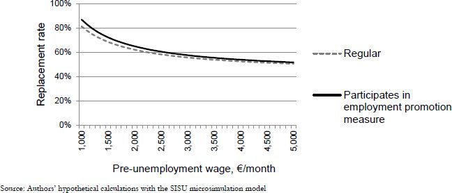
The earnings-related benefit in Finland is based on one’s pay before the unemployment spell. The benefit amount consists of the basic component (equal to the flat-rate benefit), the earnings-related component and child increases.3 As demonstrated in Figure 1, the benefit amount has no ceiling, but the replacement rate declines with higher wage.

Determination of earnings-related unemployment benefit in Finland 2017.
Source: Authors’ hypothetical calculations with the SISU microsimulation model.
3. Potential benefit duration in earlier research
There is a vast body of both empirical and theoretical literature related to labor market effects of unemployment benefits (for an older overview, see for example Krueger & Meyer, 2002). Especially North American research is plentiful, but empirical evidence is also available from Europe and the Nordic countries. More recent behavioral economic theory has paid attention specifically to the duration of unemployment benefits as a crucial factor explaining changes in re- employment rates (see DellaVigna, Lindner, Reizer, & Schmieder, 2017). Empirical evidence (ibid.) suggests that even without changing the overall generosity of the unemployment benefits, reducing the duration of benefits may increase re-employment rates.
In their review article, Tatsiramos and van Ours (2014) analyze the results of six articles, the latest being from 2012. The analyzed contexts include the US, Slovenia, Germany and Austria. The authors conclude that a PBD increase of 100 days extends the unemployment spells by 20 days on average, with some variation across countries. The benefit semi-elasticities, that is, the percentage change in unemployment duration in response to a percentage point change in the gross replacement rate, seem to range between 0.4 and 1.0.
In the US, Farber and Valletta (2015) exploit PBD reforms in different states to disentangle the causal effect. They find a small but statistically significant effect of PBD on unemployment: an increase of 100 days in the PBD resulting in an increase of six days of unemployment. Hagedorn, Manovskii, and Mitman (2015) employ the abolishment of all state level increases in the duration of the unemployment benefits. By comparing neighboring municipalities of different states, they conclude that a one percent change in the PBD results in a 1.4–2.3 percent change in employment and a 0.6–1.2 percent change in the participation rate. Furthermore, the authors estimate that the PBD cuts explain 50–80 percent of the improvement of the aggregate employment in 2014.
Because of the existence of the flat-rate scheme in Finland, the reduction in PBD can also be interpreted as a cut in the unemployment benefit level. Therefore, the literature on the benefit level changes is reviewed next. Uusitalo and Verho (2010) analyze the effects of an unemployment benefit increase using a natural experiment to identify the causal effect. They found that a 15 percent raise in the average earnings-related unemployment benefit amount reduces re- employment rates by 17 percent, elasticity being approximately 0.8.
Kyyrä and Pesola (2017) analyze the effects of unemployment benefits on unemployment exits and labor market outcomes using a method called regression kink design. According to their findings, a higher benefit level prolongs unemployment with an elasticity between 1.5 and 2. The elasticity of moving from unemployment directly to employment is found to be around −0.5. However, the results are somewhat sensitive to the choices of bandwidth and polynomial order.
Kyyrä, Pesola, and Rissanen (2017) exploit the variation in remaining benefit duration days at the beginning of subsequent unemployment spells as their causal specification. The authors find, among other things, that an additional week of earnings-related unemployment benefit increases the expected unemployment duration by 0.15 weeks.
As a summary, the empirical evidence on the effect of both the benefit level and duration on employment is largely and nearly unambiguously in line with the expectations drawn from economic theory. Changes in unemployment benefits affect the length of the unemployment spells and shorter spells in turn yield a higher aggregate rate of employment.
4. Data
All statistics and evaluations presented in this article are based on a data set of roughly 800,000 individuals, which amounts to 15 percent of the population of Finland at the end of 2014. The data are compiled on annual basis by Statistics Finland as part of the Finnish microsimulation model SISU (see Statistics Finland, 2018). The data include comprehensive information on demographic and socio-economic characteristics of population such as age, sex, family type and household income. In addition, they contain detailed information on individuals’ income from employment, social benefits and paid taxes which enable microsimulation of a majority of Finnish social benefits and taxation legislation.
PBD legislation applies to individual unemployment spells, which, according to the law, last until one fulfills the employment condition again (working for at least eight months, see Section 2 for details). However, received social security benefits are not observed in spells, but on an annual level and, therefore, do not reflect the actual cumulated length of unemployment spells. This is the case if, for instance, one has become employed during the year and consequently has two distinct unemployment spells. Therefore, the data are complemented with information on unemployment duration at the end of each quarter, which enables us to simulate the PBD legislation in detail.
Approximately 330,000 persons received earnings-related unemployment benefit in Finland during 2014. The reform divides the unemployed into three groups by their PBD instead of the previous two. After the reform, the PBD of 300 days is implemented for those with the shortest employment history. As presented in Table 2, this group constitutes eight percent of all recipients of earnings- related benefit. Three out of four unemployed have had their PBD decreased to 400 days. The PBD of the remaining 17 percent remains at 500 days or more.
The distribution of demographic and economic characteristics by duration categories.
| Potential duration (new/old) | N | % | Female % | Average age | Average work history | Average benefit €/day | Receipt of benefits % | |
|---|---|---|---|---|---|---|---|---|
| Housing benefits | Social assistance | |||||||
| 300/400 | 24,941 | 8 | 50 | 30 | 2 | 57.1 | 28 | 15 |
| 400/500 | 248,562 | 75 | 49 | 43 | 11 | 70.3 | 13 | 8 |
| 500+/500+ | 56,535 | 17 | 48 | 61 | 14 | 70.0 | 6 | 3 |
| All | 330,038 | 100 | 49 | 45 | 11 | 69.2 | 13 | 8 |
-
Notes: Information for work history is available since 1997, thus the maximum work history is 17 years. The receipts indicate simulated receipt during the year, not necessarily simultaneously with the unemployment benefit spell.
The division by PBD is determined by age and work history (see Section 2). Therefore, the average age is naturally the lowest, 30 years, in the first group and the highest, 61 years, in the last group. Correlating highly with age, the benefit levels and receipt of means-tested benefits, that is housing benefits and social assistance, are distributed in a similar way. The group with a potential duration of 300 days has clearly the lowest unemployment benefits and, consequently, receives means-tested benefits more often.
As can be seen in Figure 2, the cumulative number of unemployment benefit days before the reform had a bimodal distribution with peaks in very short spells (10 days) and at maximum duration (500+ days). There is also a small concentration at 400 days, which equals the PBD of those with a short work history.

Pre-reform distribution of cumulative days of earnings-related benefit by the end of 2014, percent of the recipients.
5. Methods
We evaluate the impact of the reform by using microsimulation of population registers (see, for example, Bourguignon & Spadaro, 2006). By calculating counterfactual benefit sums according to different legislations, we can distinguish the static impact of the reform to the individual as well as to the whole population, given that our data represents the total population.
We base our calculations on the static microsimulation model SISU (Statistics Finland, 2018), complemented with a module that enables us to calculate a behavioral change in labor supply, and also to assess behavioral change in public expenditures and income distributions. The static simulation of unemployment benefits runs as follows. First, the unemployment benefit days of both earnings-related and flat-rate schemes are simulated according to the chosen legislation. If the PBD is decreased, the number of unemployment days with earnings-related benefit is transferred to the flat-rate scheme. Then daily benefit amounts are simulated and multiplied with the number of days. Thereafter, taxation legislation and entitlement to housing benefit and social assistance are simulated.
Before we run the static simulation, we estimate the behavioral response to the unemployment spells. The typical approach of estimating a behavioral response in the context of microsimulation is first to estimate a discrete choice labor supply model that relates labor supply to the change in disposable income. However, this comes with high requirements for data and modeling. Panel data is required to credibly estimate replacement and employment rates because the cross-sectional variation is not random but subject to unobserved selection processes.
It might be possible to build a structural model that would estimate behavioral response to changes in disposable income also with cross-sectional data. This would mean trying to identify, for example, the uncompensated elasticity of labor supply using changes in disposable income between various groups in repeated cross-sections. But as our main point of interest lies within the unemployment scheme, this behavioral model would probably not capture the behavioral effect of changes in unemployment scheme. The elasticity estimated using variation in taxation is probably not identical to elasticity estimated using variation in unemployment scheme.
Here we present an alternative method that can be used when one does not have panel data and detailed information on the unemployment spells in disposal. Instead of using correlations discovered by a discrete choice model, we apply elasticities derived from external research to the specific group of interest. This allows us to use external information on causation, whereas, with the cross-sectional data available to us, a discrete choice model would possibly discover correlations between labor supply and disposable income that might not have a causal relation. The aforementioned pros and cons of using discrete choice model and external elasticities (our approach) are compiled in Table 3.
Pros and cons of the two approaches of labour supply estimation.
| Discrete choice model | External elasticities | |
|---|---|---|
| Pros | • Empirically fit for the specific context • Better accuracy |
• Light data requirement • Genuine causal relationship (however, possibly from a different population) • Transparency, simplicity |
| Cons | • Heavy data requirement • Complexity, sensitivity • Changes in PBD typically ignored |
• Elasticities subject to context-specific inaccuracy • More inaccuracy in the distributional effects |
The application of external elasticities is conducted as follows. First, we define the unemployment benefit elasticity, η:
The elasticity parameter is defined as the percentage change in unemployment duration (Dur) in response to a one percentage-point increase in benefit replacement rate (rr). As depicted in Table 1, two groups experience different changes in their PBD and one group sees no change. Therefore, the percentage point changes in the replacement rates for the three groups are the following:
where rrER denotes the replacement rate of earnings-related unemployment benefit and rrFR denotes the replacement rate in the flat-rate scheme (see Section 2).
We apply an elasticity estimate to the change in replacement rate. Another option would have been to apply an elasticity estimate to the average duration of an unemployment spell, but we depart from this approach due to practical reasons, since the data available does not allow us to directly observe the average duration of unemployment spells.
In choosing the elasticity estimate, we follow the review by Tatsiramos and van Ours (2014) who conclude that the benefit elasticity of Equation 1 ranges between 0.4 and 1.0 (see Section 3). We use the mean value of 0.7 as our baseline specification. However, we present additional results from static simulation (elasticity 0) as well as with elasticities of 0.4 and 1.0 to illustrate the sensitivity of the estimates.
It is possible that a single homogenous and constant elasticity is not realistic. We therefore introduce variation into benefit elasticity by weighting it with the predicted employment probabilities, which correlate positively with benefit elasticity.4 Resulting elasticity for individual i can be denoted:
Equation 3 captures the fact that individuals with better employment prospects also have shorter unemployment spells. The regression model used to predict the employment probabilities is reported in the Appendix. The elasticities vary from 57 percent to 147 percent of the mean elasticity, which seems a realistic assumption on the basis of the literature. To infer the role of heterogeneity, we run also a scenario with constant elasticity of 0.7. The elasticities used in different scenarios are depicted in Table 4.
The distribution of predicted employment probabilities and subsequent elasticities in different scenarios.
| Min | P10 | P25 | Median | P75 | P90 | Max | |
|---|---|---|---|---|---|---|---|
| Predicted employment probabilities | 0.30 | 0.43 | 0.48 | 0.53 | 0.58 | 0.62 | 0.78 |
| Weighted elasticities (mean = 0.4) | 0.23 | 0.33 | 0.37 | 0.40 | 0.44 | 0.47 | 0.59 |
| Weighted elasticities (mean = 0.7) | 0.40 | 0.58 | 0.64 | 0.71 | 0.77 | 0.83 | 1.03 |
| Constant elasticities (mean = 0.7) | 0.70 | 0.70 | 0.70 | 0.70 | 0.70 | 0.70 | 0.70 |
| Weighted elasticities (mean = 1.0) | 0.57 | 0.83 | 0.92 | 1.01 | 1.10 | 1.18 | 1.47 |
-
Source: Authors’ calculations.
The simulated behavioral response reflects both the demand and supply sides of the economy because the demand and supply side constraints are present in the used elasticity estimates drawn from the empirical literature (Tatsiramos & van Ours, 2014). We cannot, however, explicitly state whether the causal inference is similarly valid in economic upturn as it is in downturn. Therefore, the behavioral response should be interpreted as an average response within a business cycle. Furthermore, applying an average elasticity of Tatsiramos and van Ours (2014) may not correctly reflect the true elasticity in Finland; this concern, however, is alleviated by the fact that Uusitalo and Verho (2010) discover a benefit elasticity of similar magnitude using Finnish data.
Furthermore, as presented in Equation 3, we assume that all unemployed increase their labor supply according to their individual elasticity 𝜂i. This is equivalent to drawing a large number of realizations from the probability distribution and using the resulting frequencies as probabilities. The result can also be interpreted to reflect a long-run equilibrium of the labor market.
We apply the elasticities of Equation 3 to the individual “simulated” changes in the replacement rates of Equation 2, and further to the individual duration of within-year unemployment, which is observed in the data. The observed duration is then modified with the aid of Equation 2 using the change in the gross replacement rate and the individual semi-elasticity. The equation that connects the reform and the change in the labor supply (dE) for an individual i with legislation j is:
Finally, the employment wage used is the one that is the basis of the unemployment benefit. We assume that there is no wage-scarring effect.
6. Evaluation of the reform
Table 5 summarizes the static effect of the reform on various population subgroups. The reform would directly shorten the unemployment spells of 39,000 unemployed, which comprises 12 percent of all recipients of the earnings-related benefit. Individuals with a lower PBD, that is shorter work history, are affected approximately as much as those with a longer work history. The share of the affected is similar between sexes. However, men have a larger drop in their disposable income, both in absolute and relative terms. This reflects the differences in family types and wages.
The static reform impact is concentrated on the long-term unemployed, who are mostly located in the lowest income groups and oldest age groups. In other words, most of the current unemployed are not directly affected by the reform as their unemployment spells, as observed in the data, appear shorter than the new limit on maximum benefit duration. Around 32 percent of recipients in the lowest income decile are affected compared to the five percent in the highest decile. Both the absolute and relative decreases in disposable income are largest among deciles II and III. The impact among the very lowest decile is cushioned by the increase of the means-tested housing benefit and social assistance.
The reform affects only seven percent of the unemployed in the youngest age group (18–25) and 16 percent of the unemployed aged 46–57 years. Most of the unemployed above the age of 58 are exempt from the reform — only three percent are affected. Both the absolute and relative decreases of disposable income are largest in older age groups.
When examined by family type, the reform concerns single adult households the most. Couples without children in their household are affected the least. Single parents in turn are affected most often. This is an interesting observation, as earlier research shows that single parents are also facing the weakest financial incentives to work in Finland (see Kotamäki, 2016).
The static effect of the reform in subgroups of recipients of earnings-related unemployment benefit.
| Unaffected, N | Affected, N | Affected, % | ∆ Disp. inc, €/year | ∆ Disp. inc, % | ||
|---|---|---|---|---|---|---|
| All | 290,778 | 39,260 | 11.9 | −479.9 | −3.2 | |
| Potential duration | 300/400 days | 20,725 | 4,216 | 16.9 | −315.7 | −2.3 |
| (new/old) | 400/500 days | 213,325 | 35,044 | 14.1 | −499.6 | −3.3 |
| 500+ days | 56,728 | 0 | 0.0 | |||
| Sex | Male | 149,319 | 20,345 | 12.0 | −602.4 | −4.1 |
| Female | 141,460 | 18,914 | 11.8 | −348.1 | −2.2 | |
| Decile | I | 12,287 | 5,828 | 32.2 | −428.3 | −4.3 |
| II | 24,774 | 6,847 | 21.7 | −645.6 | −4.9 | |
| III | 31,281 | 6,100 | 16.3 | −692.4 | −4.7 | |
| IV | 34,531 | 4,815 | 12.2 | −518.6 | −3.1 | |
| V | 36,222 | 4,156 | 10.3 | −449.8 | −2.4 | |
| VI | 36,562 | 3,523 | 8.8 | −252.7 | −1.2 | |
| VII | 35,869 | 2,818 | 7.3 | −320.6 | −1.4 | |
| VIII | 32,626 | 2,378 | 6.8 | −302.9 | −1.1 | |
| IX | 29,077 | 1,871 | 6.0 | −223.6 | −0.7 | |
| X | 17,548 | 926 | 5.0 | −435.1 | −0.9 | |
| 18−25 | 18,294 | 1,299 | 6.6 | −222.1 | −1.7 | |
| 26−35 | 62,895 | 9,164 | 12.7 | −365.9 | −2.5 | |
| 36^5 | 60,064 | 10,656 | 15.1 | −466.4 | −2.9 | |
| 46−57 | 82,974 | 16,023 | 16.2 | −562.6 | −3.7 | |
| 58− | 66,551 | 2,118 | 3.1 | −573.3 | −4.2 | |
| Family type | Single dweller | 66,664 | 10,283 | 13.4 | −941.8 | −6.8 |
| Single parent | 18,747 | 3,703 | 16.5 | −670.8 | −3.5 | |
| Couple | 104,205 | 10,949 | 9.5 | −282.7 | −1.9 | |
| Couple w/ | ||||||
| children | 95,348 | 13,060 | 12.0 | −202.3 | −1.0 |
-
Source: Authors’ calculations.
-
Notes: The mean changes in disposable income are in equivalent household disposable income among the affected, euros in the 2016 price level.
The above description addresses the static, i.e. the immediate effect of the reform in subgroups. In the following, we consider the behavioral response jointly with the static effect. Five scenarios with mean elasticities of 0.0, 0.4, 0.7 and 1.0 are presented. For 0.7, scenarios with heterogeneous and constant elasticities are presented; the heterogeneous one being the baseline.
In Table 6, we present the estimated effects of the reform distinctly on different income units such as the two unemployment benefit schemes, wage sum, tax revenue and means-tested benefits as well as the total impact on fiscal and household budgets. In all scenarios, the cut in the PBD of the earnings-related benefit is cushioned by the flat-rate unemployment benefit scheme, taxation and the means-tested benefit. It logically follows from our assumptions that the wage sum increases in scenarios, which accounts for the behavioral response.
In the government bill, the reform was expected to cut EUR 159 million from the earnings-related unemployment benefit expenditure. The static estimate presented in Table 6 is somewhat close to the target, EUR 175 million. The baseline behavioral effect, calculated with the elasticity of 0.7, exceeds the expected figure by EUR 50 million. In the static scenario, more than half of the expenditure decrease observed in the earnings-related scheme is mirrored back in the flat-rate scheme. However, the expenditure increase of the flat-rate scheme is smaller in scenarios where the behavioral response is taken into account.
The effects of the reform on different income units by benefit elasticities, million euros in 2016 price level.
| Pre-reform total | 0.0 (static) | 0.4 | A, by elasticity 0.7 (baseline) | 0.7 (constant) | 1.0 | |
|---|---|---|---|---|---|---|
| Earnings-related scheme | 2,558 | −175 | −193 | −209 | −209 | −225 |
| Flat-rate scheme | 1,517 | +94 | +83 | +75 | +75 | +68 |
| Wage sum | 80,466 | +0 | +66 | +118 | +119 | +169 |
| Taxes | 33,275 | −25 | −19 | −12 | −11 | −4 |
| Housing benefits | 2,103 | +7 | +6 | +6 | +6 | +6 |
| Social assistance | 1,003 | +3 | +2 | +2 | +1 | +1 |
| Total, fiscal | +48 | +83 | +115 | +115 | +146 | |
| Total, households | −48 | −17 | +3 | +4 | +22 | |
| Unemployment days | 91,700,229 | 0 | – | −1,027,728 | −1,028,853 | – |
| 575,876 | 1,465,234 |
-
Source: Authors’ calculations.
The cuts in unemployment insurance in total result in a decrease of tax revenue. The effect on tax revenue remains negative but diminishes when the behavioral response is taken into account and tax revenue from employment starts to increase. Housing benefits and social assistance increase slightly less when the behavioral response is taken into account. Overall, the positive effect on public finances more than doubles in the baseline behavioral scenario compared to the static scenario.
The scenarios with heterogeneous and constant elasticities demonstrate negligible mean differences. Closer examination reveals that this results from relatively weak correlations between estimated employment probabilities and unemployment duration as well as the changes in replacement rates (see Equation 4). However, when tabulated by subgroups such as age or education (not shown), some differences emerge. For instance, unemployed younger than 27 years of age demonstrate an eight percent greater decrease in their unemployment spells in the scenario with heterogeneous elasticities.
As depicted in Table 7, the reform is estimated to result in a very marginal increasing effect on most inequality indicators. In the static scenario, the Gini index increases by 0.02 and the general at-risk-of-poverty rate by 0.03 percentage points. The median equalized income in the total population decreases marginally, which causes the relative poverty risk among the elderly, who are otherwise unaffected by the reform, to decline.
The effects of the reform on inequality indicators by benefit elasticity.
| Pre-reform total | 0.0 (static) | 0.4 | ∆ by elasticity 0.7 (baseline) | 0.7 (constant) | 1.0 | ||
|---|---|---|---|---|---|---|---|
| Gini index | 26.64 | +0.02 | +0.01 | +0.01 | +0.01 | 0.00 | |
| At-risk-of poverty, % | All | 12.98 | +0.03 | +0.02 | +0.02 | +0.01 | +0.01 |
| (60) | < 18 yrs | 11.88 | +0.03 | +0.03 | +0.03 | +0.03 | +0.02 |
| > 65 yrs | 13.08 | −0.02 | 0.00 | +0.02 | +0.02 | +0.03 | |
| Median income (€/year) | 23 820 | −12 | −3 | +4 | +4 | +8 |
-
Source: Authors’ calculations.
The inclusion of the behavioral effect in the estimation reduces the small static increase in the Gini coefficient. A similar pattern is also visible among the poverty risk indicators. The at-risk-of- poverty estimates increase less in the baseline behavioral scenario compared to the static simulation.
Finally, we observe only marginal change in income inequality measured by the Gini index in the baseline scenario. Similarly, changes in the at-risk-of-poverty indicators are smaller in the baseline behavioral scenario. Respectively, with lower elasticities the inequality effects are more visible. Again, no decisive differences emerge when used constant elasticities. The changes of all indicators, however, are very small in all scenarios.
7. Conclusions
In this study, we estimated the ex-ante effects of a 2017 reform that cut the potential benefit duration of the earnings-related unemployment benefit by 100 days in Finland. Instead of using correlations discovered by a discrete choice model, we apply external elasticities derived from microeconomic research to the specific group of interest. We argue that this approach is useful in situations like ours when the estimation of a discrete choice model is difficult, for example when sufficient data is unavailable.
Our main results are as follows. The static simulation results in a net cut of EUR 81 million in unemployment-related expenditures and EUR 48 million overall, after accounting for taxes and other benefits. Incorporating behavioral effects changes the estimates drastically. The overall behavioral fiscal effect is +EUR 115 million and +EUR 3 million for the households given a benefit elasticity of 0.7. The positive fiscal effect more than doubles and the negative effect on household income seen in the static scenario turns positive.
A similar pattern is visible in inequality indicators. We observe that the PBD cut marginally increases the income inequality measured by the Gini index when the behavioral response is not included in the model. However, the inclusion of the behavioral response reduces this increase; we observe a smaller change in the Gini index when the increase in employment with 0.7 elasticity is considered.
We introduce heterogeneity in the elasticities by weighting them with estimated employment probabilities. However, this method produces almost identical inequality indicators as the simulation with constant elasticities. The result can hardly be generalized to other contexts. It is likely that reforms with more decisive inequality effects would show greater differences between the two approaches.
Overall, the static simulation of the reform gives a somewhat pessimistic and modest picture of the reform. Including the behavioral response improves the picture from all perspectives: fiscal budget, household income as well as inequality. Our example of the Finnish unemployment insurance reform shows that higher benefit elasticities can indeed result in more favorable distributional effects. This finding leads to a policy recommendation that benefit cuts should be targeted towards population groups with high benefit elasticity to minimize the increase in inequality.
Footnotes
1.
We use the term “behavioral microsimulation” when referring to microsimulation analysis that takes labor supply response into account.
2.
A large majority of employees in Finland are members of unemployment funds. In 2016, the membership fees varied between € 23 and 174/year or 0.18 and 3.7 percent of yearly gross wage. The benefit is administered and paid by the unemployment funds of which there were 28 in 2016. The number of unemployment funds has been in a declining trend for quite some time. (Finnish Financial Supervisory Authority, 2017.)
3.
The amount of the basic component is € 32.40 per day in 2017. The earnings-related component is 45 percent of the difference between the daily pay and the basic component up until a monthly wage level of €3,078 in 2017 after which the earnings-related component is 20 percent of the exceeding amount. Moreover, in 2017, individuals can also receive increased allowance if they participate in employment promoting measures. The increased earnings-related allowance is 55 percent of the difference between the daily pay and the basic component up until €3,078 after which the percentage is 25. Child increases are paid for children less than 18 years of age. Child increases amount to €5.23, 7.68 and 9.90 per day for one, two and three children. The unemployment benefits are taxable income, with a tax rate starting from 20 percent and slightly increasing as the benefit level increases.
4.
Formally, this can be seen as follows: following empirical labor economic literature, assume that the probability of employment (p(a)) is exponentially distributed: p(a)=1-exp(-r*a), where a is search effort and r is the parameter that governs labor supply elasticity. It is evident that the probability of employment and labor supply elasticity have a positive association with any given level of search effort: dp(a) = exp(-r*a)*a dr, dr>0. The duration of employment is given by 1/p(a), which implies that a higher probability of employment, or, higher labor supply elasticity leads to shorter duration of unemployment.
Appendix
1. Predicting the employment probabilities
The estimated regression equation is given by:
where β denotes the vector of regression coefficients, X denotes the vector of explanatory variables and the logistic function of E is given by
By exploiting the unemployment information at the end of 2013, we can deduce the possible event of employment in 2014. Therefore, we concentrate the estimation on those who have been unemployed at the turn of the year (n = 15,975) and extend the prediction of employment probability to all unemployed in the earnings-related scheme. The binary event of employment (e) is defined as follows:
Regression coefficients are reported in Table A.1 and the distribution of predicted employment probabilities in Table 4.
Results from the logistic regression modelling employment probability (n = 15,975).
| Goodness of fit criterion | Intercept only | Intercept and covariates | ||||
|---|---|---|---|---|---|---|
| AIC | 22,101 | 21,836 | ||||
| SC | 22,108 | 22,097 | ||||
| −2 Log L | 22,099 | 21,768 | ||||
| Coefficient | (S.E.) | OR | ||||
| Intercept | 0.037 | (0.172) | 1.038 | |||
| Education | ||||||
| No post-basic level education or | ref | |||||
| level of education unknown | ||||||
| Upper secondary education | 0.246 | (0.050) | 1.128 | |||
| Lowest level tertiary education | 0.150 | (0.058) | 1.162 | |||
| Higher tertiary or doctorate level | 0.190 | (0.071) | 1.210 | |||
| Number of children | ||||||
| 0 | ref | |||||
| 1 | ||||||
| 2 | −0.032 | |||||
| −0.093 | (0.053) (0.074) | 0.968 0.911 | ||||
| >2 | −0.327 | (0.158) | 0.721 | |||
| Sex | ||||||
| Male | ref | |||||
| Female | −0.125 | (0.033) | 0.882 | |||
| Coresidence status | ||||||
| Single dweller | ref | |||||
| Couple | 0.288 | (0.035) | 1.334 | |||
| Age | ||||||
| < 25 | ref | |||||
| 25–29 | −0.264 | (0.172) | 0.768 | |||
| 30–34 | −0.362 | (0.168) | 0.696 | |||
| 35–39 | −0.373 | (0.168) | 0.689 | |||
| 40–44 | −0.447 | (0.167) | 0.639 | |||
| 45–49 | −0.495 | (0.166) | 0.610 | |||
| 50–54 | −0.582 | (0.166) | 0.559 | |||
| > 55 | −0.709 | (0.166) | 0.492 | |||
| Region | ||||||
| Uusimaa | ref | |||||
| Varsinais-Suomi | 0.154 | (0.064) | 1.167 | |||
| Satakunta | 0.209 | (0.079) | 1.233 | |||
| Kanta-Hame | 0.372 | (0.104) | 1.451 | |||
| Pirkanmaa | 0.144 | (0.062) | 1.154 | |||
| Paijat-Hame | 0.289 | (0.088) | 1.336 | |||
| Kymenlaakso | 0.412 | (0.088) | 1.510 | |||
| South Karelia | 0.193 | (0.109) | 1.212 | |||
| Etela-Savo | 0.326 | (0.102) | 1.385 | |||
| Pohjois-Savo | 0.507 | (0.081) | 1.660 | |||
| North Karelia | 0.311 | (0.089) | 1.365 | |||
| Central Finland | 0.283 | (0.071) | 1.327 | |||
| South Ostrobothnia | 0.651 | (0.094) | 1.918 | |||
| Ostrobothnia | 0.359 | (0.108) | 1.432 | |||
| Central Ostrobothnia | 0.231 | (0.156) | 1.260 | |||
| North Ostrobothnia | 0.346 | (0.064) | 1.413 | |||
| Kainuu | 0.397 | (0.107) | 1.487 | |||
| Lapland | 0.408 | (0.083) | 1.503 | |||
| Aland | 0.383 | (0.414) | 1.466 | |||
-
Source: Authors’ calculations with the research data.
References
-
1
The distributional effects of fiscal consolidationThe distributional effects of fiscal consolidation, IMF Working Paper No. 151, Washington, D.C., International Monetary Fund.
-
2
Comparing labor supply elasticities in Europe and the United States: new resultsJournal of Human Resources 49:723–838.
-
3
Microsimulation as a tool for evaluating redistribution policiesJournal of Economic Inequality 2006:77–106.
-
4
Discrete hours labour supply modeling: specification, estimation, and simulationJournal of Economic Surveys 19:697–734.
-
5
Income distribution in discrete hours behavioural microsimulation models: An illustrationJournal of Economic Inequality 4:57–76.
-
6
The effect of tax-benefit changes on the income distribution in 2008-2014The effect of tax-benefit changes on the income distribution in 2008-2014, EUROMOD Working Paper No. 11),, Colchester: University of Essex.
-
7
Reference-dependent job search: evidence from HungaryThe Quarterly Journal of Economics 132:1969–2018.
-
8
Do extended unemployment benefits lengthen unemployment spells? Evidence from recent cycles in the US labor marketJournal of Human Resources 50:873–909.
-
9
http://ec.europa.eu/eurostat/statistics-explained/index.php/Employment_statisticsEmployment statistics..
- 10
-
11
The Impact of Unemployment Benefit Extensions on Employment: The 2014 Employment Miracle?. NBER Working Paper No. 20884Cambridge: National Bureau of Economic Research.
-
12
Participation tax rates in Finland, earned-income tax credit investigated. Aboa Centre for Economics Discussion Paper No. 107Turku: Aboa Centre for Economics.
- 13
-
14
The Effects of UI Benefits on Unemployment and Subsequent Outcomes: Evidence from a Kinked Benefit Rule. (IZA Discussion Paper No. 10484Bonn: Institute of Labor Economics.
-
15
Unemployment Insurance in Finland: A Review of Recent Changes and Empirical Evidence on Behavioral Responses (VATT Research Reports No. 184)Helsinki: VATT Institute for Economic Research.
-
16
A Structural Analysis of Labour Supply Elasticities in the Netherlands. CPB Discussion Paper No. 235Amsterdamml: Netherlands Bureau for Economic Policy Analysis.
-
17
http://www.stat.fi/tup/mikrosimulointi/index_en.htmlThe description of the SISU microsimulation model.
-
18
Labor market effects of unemployment insurance designJournal of Economic Surveys 28:284–311.
-
19
The effect of unemployment benefits on re-employment rates: Evidence from the Finnish unemployment insurance reformLabour Economics 17:643–654.
-
20
Distributional consequences of fiscal consolidation and the role of fiscal policy: What do the data say? IMF Working Paper No. 195Washington, D.C.: International Monetary Fund.
Article and author information
Author details
Acknowledgements
We would like to state our gratitude to Henri Keränen, Allan Seuri and Olli Kannas for useful comments. In addition, we would like to remind that we do not represent the official views of our background organizations.
Publication history
- Version of Record published: August 31, 2018 (version 1)
Copyright
© 2018, Kotamäki et al.
This article is distributed under the terms of the Creative Commons Attribution License, which permits unrestricted use and redistribution provided that the original author and source are credited.