Accounting for tax evasion profiles and tax expenditures in microsimulation modelling. The Betamod model for personal income taxes in Italy
- Ca’ Foscari University, Italy
- Article
- Figures and data
-
Jump to
- Abstract
- 1. Introduction
- 2. The micro database and related imputations
- 3. The construction of Betamod
- 4. Validation and main results
- 5. Tax evasion and its distributional profile
- Footnotes
- A. Statistical matching between the IT-SILC and SHIW datasets
- B. Estimation of tax evasion rate
- C. Incidence of tax reliefs on reported income
- References
- Article and author information
Abstract
The paper presents the main characteristics of Betamod, a static microsimulation model that reproduces the Italian personal income tax (Irpef), as well as local income taxes, namely the regional and municipal surtaxes, building on a detailed reconstruction of tax legislation. With respect to the vast majority of existing tax microsimulation models, the peculiarities of Betamod concern two aspects: the inclusion of a detailed set of tax expenditures, and the estimation of individual-specific tax evasion rates, which account for the total individual income level, its composition in terms of income sources, and the geographical area of residence.
1. Introduction
Tax-benefit microsimulation models have become a standard tool for the design and the evaluation of public policies in many countries (see, among others, Bourguignon & Spadaro, 2006; Mitton, Sutherland & Weeks, 2000; Sutherland & Figari, 2013). Indeed, devising effective policy interventions requires appropriate ex-ante evaluation instruments, not only informative about the macro-level revenue consequences, but also about the distributional outcomes of specific interventions. In this respect, and particularly in a single-country framework, the accuracy of a particular model in accounting for aspects that are more salient in the national context, or the object of planned reform interventions, is key to its predictive power and, therefore, relevance.
In the Italian context, two aspects currently deserve particular attention. The first is tax evasion, which is extremely high, i.e. estimated in the range of 18–25% of Gdp in terms of unreported incomes (Giovannini, 2011). Various political leaders, as well as a significant share of the public opinion, seem to justify tax evaders on the grounds that tax rates are too high and the tax schedule far too progressive. At the same time, the distributional consequences of tax evasion are often neglected in the public discourse, or dismissed with generic statements based more on anecdotal evidence than grounded empirical analysis. For example, little is known about the distinct effects that tax evasion may bear to progressivity (vertical effect) versus horizontal equity and re-ranking (Aronson & Lambert, 1994; Urban & Lambert, 2008). Microsimulation models have a major potential in this respect. The second aspect is that of tax expenditures. Over the last decade, tax expenditures in Italy have consistently increased as a share of Gdp. Recently, the Italian Ministry of Economy and Finance identified 720 measures of tax expenditures that account for about the per cent of Gdp (Keen et al., 2012). Among these, the individual income tax expenditures are the largest (4.84% of Gdp). Because of the entailed reduction in tax revenues, and the induced distortions in taxpayers’ behavior, there is an increasing debate, both at the national and international level, on the use of tax expenditures as alternative to direct expenditures (e.g. see Avram, 2014; Burman, 2003; Burman et al., 2008; Poterba, 2011; Tyson, 2014), also on the grounds of their regressive effect (e.g. Matsaganis & Flevotomou, 2007).
This paper presents a new microsimulation model, called Betamod, for the Italian personal income tax (Irpef), including also local income taxes, namely the regional and municipal surtaxes, which tackles these two aspects. In more detail, Betamod improves on the existing Italian models1 by estimating a distribution of individual tax evasion rates, based on total individual income level, its composition in terms of sources, and geographical area. With respect to other Italian models, where tax evasion rates are assumed to be constant within population subgroups (e.g. by income source type, by income classes), Betamod, assigns a tax evasion rate to each individual. This allows to evaluate more accurately how tax evasion may alter the redistributive effect of personal income taxation, and to measure the horizontal, vertical and re-ranking effects, each of which is possibly altered by tax evasion. Moreover, Betamod accounts thoroughly for a detailed set of tax allowances and tax credits. Compared to the majority of current microsimulation models for Italy, Betamod includes all kinds of individual income tax expenditures and allows us to estimate the distributional effects of all tax expenditures simultaneously and of specific tax reliefs or categories of expenditure in turn.
The paper is organized as follows. Section 2 describes the data set and the preliminary data adjustments and imputations required to simulate accurately the Italian personal income taxes. Section 3 illustrates, in details, the process of constructing Betamod, focusing in particular on its innovative aspects. With reference to the 2010 fiscal year, Section 4 tests the robustness of the model by comparing the baseline simulation of personal income tax and local income taxes with official figures provided by tax returns data. Finally, Section 5 provides novel distributional evidences on tax evasion and on its profile, as well as on individuals’ re-ranking between income classes resulting from it2.
2. The micro database and related imputations
Betamod runs on the Italian national version of the Survey of Income and Living Conditions (It-Silc), which represents, with a few exceptions, the micro-database currently chosen by most tax- benefit microsimulation models for Italy3. With respect to the alternative Survey on Households Income and Wealth (Shiw), It-Silc takes the advantage of a more generous sample size (19,399 households in It-Silc versus 7,951 households in Shiw), allowing to conduct analyses by geographical area sample; the drawback of this choice is the lack of information on household’s assets and tax-relevant expenditures.
We use the cross-sectional component of It-Silc 2011, which features a considerably larger sample size than the rotating longitudinal component. The interview is structured into an household level questionnaire, collecting information on household composition, accommodation, housing costs, and economic circumstances (including savings, debts, receipt of family-related and means-tested benefits and children’s incomes); and an individual level questionnaire, which is administered to all household members aged 16 years old or above. In the individual level questionnaire, besides information on education, health and occupation, detailed information on individual’s income from various sources relevant for tax base assessment (employment, self-employment, old age and disability pensions, incapacity and disability benefits, rents from properties, investment income and other incomes) is covered. For income components subject to taxation4, the amount as net of taxes (and of social insurance contributions, where applicable) is collected, because net amounts are generally regarded as less exposed to measurement error and recall bias than gross ones. Reflecting the structure of the Italian fiscal system, where incomes earned in the solar year t are taxed in the following (t+1), the reference period in income-related questions is the previous fiscal year, that is 2010. This represents a mismatch with respect to demographic information, which reflects the situation of households at the time when the fieldwork was carried out (i.e. March and April 2011), and which has therefore been brought backward to 2010.
Still, an accurate simulation of Italian personal income tax requires additional information with respect to It-Silc topics coverage. Most notably, the personal income tax base includes not only employment and self-employment income, replacement income, profits from non-corporate enterprises and a marginal part of investment income, but also figurative income on immovable properties, valued as cadastral rent5, which is not covered in the survey. Besides, information on specific items of expenditures (e.g. healthcare, house refurbishments, etc.) that are relevant for specific tax reliefs, are not available in It-Silc. Missing information has therefore been imputed, drawing from other population-representative surveys covering the subject domains of interest.
We use the 2010 Survey on Households Income and Wealth released by the Bank of Italy (Bank of Italy, 2012), for imputing information on the self-reported asset value6 of the main residence, and other immovable properties, used to compute cadastral values. Drawing from the same survey, we also impute insurance premiums and house refurbishments expenditures, relevant for the computation of specific, and quantitatively important, tax reliefs. Imputation from Shiw has been performed using statistical matching techniques, where Shiw individuals have acted as ‘donors’ of the otherwise missing information for It-Silc observed ‘recipients’. Matching aims at selecting, for each It-Silc recipient, the Shiw donor that is closest to observational identity, i.e. the most similar in terms of characteristics, observed in both surveys that are predictive of the variable to be imputed. The quality of the matching procedure relies crucially on a so-called common support requirement of overlapping in the distribution of predictive characteristics in the donors’ and recipients’ samples, which has been empirically tested. The matching procedure we have adopted is based on a combination of stratification and Mahalanobis distance nearest neighbor algorithm (Rubin, 1980). Matching has been performed at the household level and with replacement, that is allowing the same Shiw household to act as donor for multiple It-Silc households, if deemed as the most adequate, rather than being discarded after having served once as donor. The donors’ and recipients’ samples have been stratified by main residence homeownership, other properties homeownership and geographical area, so that exact matching on these variables is ensured; then, within each stratum, the donor household has been selected based on the Mahalanobis distance metric, measured on other predictive variables. These include equivalent household income, the percentage of household members with more than upper secondary educational qualification, a set of household composition dummies, and the main earner’s employment status. The quality of matching has been gauged by investigating the balance (e.g. in terms of equality in means) in predictive variables between recipients and matched donors, and the procedure adjusted as long as achieved balance was deemed unsatisfactory. More detail on the implementation of the matching- based imputation, and the achieved balance, is reported in Appendix A.
As a result of the matching-based imputation from Shiw data, information on the asset value of owned properties is integrated into It-Silc. However, for fiscal purposes, properties are valued in terms of cadastral rental values. Therefore, we build on existing Land Registry data, which provide information on the distribution of properties values and corresponding cadastral incomes (separately by gender, by age group, by household composition, by marital status, by geographical area and by main residence/secondary property) to derive a measure of cadastral income from the available information on properties asset values, integrated into It-Silc. For assessing the cadastral value of the main residence, Land Registry information on the ratio between asset value and cadastral income is first of all expanded, using the Ras methodology7, to obtain marginal distributions across 300 subgroups, defined in terms of the above mentioned variables. After the It-Silc sample has been correspondingly stratified, the cadastral value for It-Silc households is computed as the ratio between the asset value of the main residence imputed from Shiw, divided by the corresponding asset-value-to- cadastral-income ratio8, drawn from the expanded Land Registry statistics. A similar procedure is followed for imputing the cadastral value of secondary properties, where appropriate9.
As an additional micro-data source, we use the 201310 Multiscopo Survey on Health Conditions and the Use of Health Services, released by the National Statistical Office (Istat, 2014), to impute information on healthcare expenditures, necessary to compute other major tax reliefs, namely those that involve the largest share of taxpayers. The Multiscopo survey has been used to estimate, at the individual level, the conditional probability of incurring in tax-relevant healthcare expenditures, such as specialists visits, drugs purchases, medical tests and treatments, as a function of predictive characteristics observed again both in Multiscopo and in It-Silc. These include gender, six age groups, self-assessed health, reported chronic conditions, limitations in activities of daily living, geographical regions, marital status, occupation, education, presence of dependent children and household size11. The estimated parameters have then been used to predict the probability of incurring in health expenditures for individuals observed in the It-Silc sample, based on their characteristics. As illustrated in the later Section 3.1, the estimated probability of healthcare spending is then flexibly used, together with fiscal data on tax reliefs, to identify beneficiaries of healthcare tax reliefs, and to impute related expenditure amounts.
3. The construction of Betamod
After the preliminary data adjustments and the imputations, the model has been built through 4 modules, integrated in an iterative procedure where outer loops (identifying recipients of tax expenditures, building calibration weights, computing individual- and income-specific tax evasion rates) feed into the inner loop of net-to-gross conversion, as depicted in Figure 1.
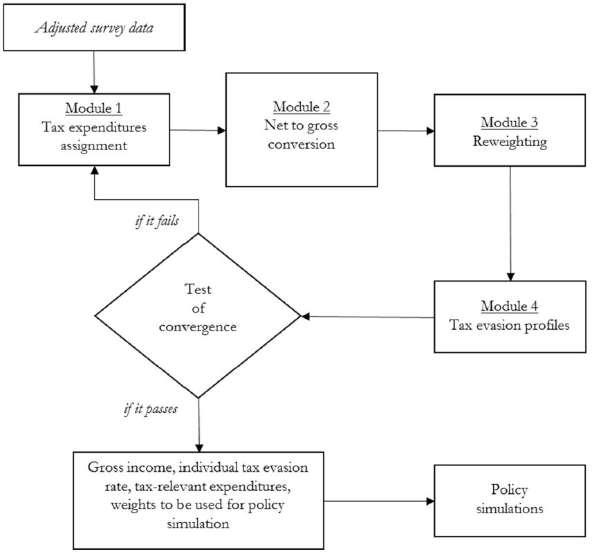

The construction of Betamod.
In more detail, based on family and personal characteristics relevant for eligibility, Module 1 identifies round-specific beneficiaries and expenditure amounts for all of the non-simulated tax reliefs, calibrating them to obtain the totals and the income distribution for beneficiaries and expenditures resulting from administrative tax returns data. Module 2 deals with the net-to-gross income conversion, through a standard iterative algorithm. Once gross and reported income measures have been obtained, Module 3 estimates calibration weights in order to match both population totals and administrative taxpayers counts. By comparison of the grossed-up obtained income measures with disaggregated administrative tax returns data, Module 4 produces an individual tax evasion rate which accounts for the individual’s different income sources composition (employment income, pensions, self-employment income12, rental income from immovable property), the income level, and geographical residence (North-West, North-East, Center, South). After Module 4, round-specific convergence, measured in terms of equality between reported incomes as estimated by the model13 and as resulting from official tax returns data14 (both at the aggregate level, and by subgroups defined by main source of income and by geographical area), is assessed.
The overall iterative procedure, continues until convergence is achieved. Specifically, the iterations stop when the reported levels of income estimated by the model, reflecting estimated tax allowances, tax evasion rates and calibration weights, not differ significantly from official tax returns data, both at the aggregate level and by subgroups (defined by main source of income and geographical area). The overall procedure generates a battery of individual level variables, including true gross income, tax evasion rate, reported income, tax relevant expenditures, calibration weights, for later use in policy simulation modelling. The following sections provide in more detail the four modules and innovative aspects of the model construction.
3.1 Deductions and tax credits module
In the Italian fiscal system there are different kinds of deductions and tax credits. The most sizeable, collectively worth over 5 per cent of Gdp, are listed in Table 1, while a comprehensive list of tax reliefs, and their quantitative importance, is reported in Tables 7 and 8. In terms of design, all deductions and tax credits are non-refundable, with the only exception of the tax credit granted to families with four children. Typically, an upper threshold applies to most tax expenditures (mortgage interest payments, rent paid by tenants, education), while the healthcare tax credit is allowed on expenses in excess of a lower threshold. Also, a withdrawal rate often applies, so that the fiscal benefit is decreasing in individual’s gross income15.
The largest PIT deductions and tax credits (fiscal year 2010).
| Description | (Value millions of Euros) | Number of beneficiaries (thousands of persons) | percent of Gdp |
|---|---|---|---|
| Deductions | |||
| Social insurance contributions paid by selfemployed individuals | 17,603 | 11,991 | 1.13 |
| Cadastral value of the main residence | 8,283 | 17,166 | 0.53 |
| Voluntary contributions to private pension plans | 1,905 | 822 | 0.12 |
| Tax credits | |||
| Tax credit for specific income sources | 41,887 | 36,426 | 2.70 |
| Tax credit for dependent family members | 11,375 | 12,624 | 0.73 |
| Tax credit for healthcare expenditures | 2,585 | 15,002 | 0.17 |
-
Source: Ministry of Economy and Finance, http://www1.finanze.gov.it/analisi_stat/index.php?tree=2011
Among deductions, the most relevant in terms of number of recipients and lost revenue, are social insurance contributions paid by self-employed individuals16, the cadastral value of the main residence and voluntary contributions to private pension plans. Other deductions are granted for specific expenditures, including legal alimony payments to spouses, donations to religious institutions, personal care services and disability aids for the disabled, and social insurance contributions paid for domestic help.
Among tax credits, the largest single item is a universal tax credit granted for specific income sources: the tax credit is applicable for either employment income, or self-employment income, or pension income, with a withdrawal rate resulting in a decreasing credit as gross income increases. This tax credit contribute to the income tax progressivity design, even more so given the absence of a legislated no tax area or legal zero rate tax bracket. Another set of tax credits aims at accounting for individual’s ability to pay, given her/his household composition (i.e. presence of dependent household members) and her/his children characteristics, such as age and disability. These tax credits are decreasing in individual gross income and become zero above a certain income threshold. The children tax credit amount and income threshold depend also on the number of children, and increase for each child aged three years or below and for disabled children. An additional refundable tax relief is granted for taxpayers with at least four children. Further tax credits are granted for specific expenditures, and amount to the 19 per cent of such expenditures: these include mainly healthcare, mortgage interest payments on both the main residence and other properties, life insurance premiums, secondary and tertiary education, childcare and charitable donations. Finally, a tax credits for up to a maximum of 55 per cent of the expenses incurred for energy conservation’s interventions and house refurbishments, and a lump sum tax credit for rent paid by low-income tenants, are allowed.
As standard in other tax benefit models for the Italian system, and reflecting data availability constraints, Betamod fully simulates the deduction for main residence cadastral value, and the tax credits by income source and for dependent family members17. However, with respect to other Italian models, which typically18 impute tax expenditures though calibration with aggregate fiscal data by income classes, Betamod calibrates not only expenditure amounts, but also beneficiaries. In particular, we aim at achieving a more realistic identification of beneficiaries, for each specific type of tax expenditure item, based on household and personal characteristics relevant for eligibility. Table 2 and Table 3 report the individual and family characteristics we used to identify the potential beneficiaries of deductions and tax credits. Simulated and non-simulated tax reliefs include all of the current categories provided by tax rules, namely, 8 deductions and different types of tax credits, these last grouped into 17 main categories. Thus, the model offers a complete picture of the wide array of tax reliefs that are part of the Italian income tax.
Deductions: identification of potential beneficiaries.
| Deductions | Potentially beneficiaries | Data source |
|---|---|---|
| Social insurance contributions paid by self-employed individuals | having self-employed income | It-Silc |
| Cadastral value of the main residence | be the owner’s of main residence | It-Silc |
| Voluntary contributions to private pension plans | those who reported to pay contributions to private pension plans | It-Silc |
| Legal alimony payments for spouse | those who reported to pay alimony | It-Silc |
| Personal care services and disability aids | identified by the estimated probability of healthcare spending | Multiscopo |
| Social insurance contributions paid for domestic help | i) presence of children
ii) having health care expenses |
It-Silc |
| Donations to religious institutions | (*) | It-Silc |
| Others | (*) | It-Silc |
-
Note: (*) Due to lack of information in the data, beneficiaries are mainly identified among the taxpayers with the higher probability of receiving other tax advantage; this is motivated by anecdotal evidence that the probability of claiming specific tax reliefs increases in the number of other tax reliefs claimed. In order to increase variance some beneficiaries have been randomly chosen
Tax credits: identification of potential beneficiaries.
| Deductions | Potentially beneficiaries | Data source |
|---|---|---|
| 19% tax credits | ||
| Healthcare expenses | identified by the estimated probability of healthcare spending | Multiscopo |
| Mortgage interest payments on main residence | i) be the homeowner’s of main residence
ii) have a mortgage loans for the purchase of the main residence |
It-Silc |
| Life insurance premium | he/she have life insurance expenses | Shiw |
| Secondary and tertiary education | i) he/she is studying
ii) have children attending high school or university |
It-Silc |
| Funeral expenses | (*) | It-Silc |
| Mortgage interest payments on other properties | i) be the homeowner’s of main residence and other properties | It-Silc |
| Annual enrollment to sports facilities | i) he/she is doing sport
ii) have children between 6 and 18 |
It-Silc |
| Rent for resident students | have children attending university and not living within the same residence as the referent individual | It-Silc |
| Social/community/home care expenses | identified by the estimated probability of healthcare spending | Multiscopo |
| Charitable donations | (*) | |
| Real estate brokerage expenses | i) be the homeowner’s of main residence
ii) have a mortgage loans for the purchase of the main residence or others properties |
It-Silc |
| Others | (*) | |
| 55% tax credits | ||
| For energy conservation’s interventions | i) be the homeowner’s of main residence
ii) have expenses for energy conservation’s interventions |
It-Silc Shiw |
| 41%-36% tax credits | ||
| House refurbishments | i) be the homeowner’s of main residence
ii) have expenses for the refurbishment of buildings |
It-Silc |
| 20% tax credits | (*) | |
| Lump sum tax credit | ||
| For tenants subject to controlled rent and for employees relocating closer to work | i) be for rent
ii) have gross income less than € 30,987.41 iii) having age between 20 and 30 years old and gross income less than € 15,493.71 |
It-Silc |
| Security sector tax credit | i) be employee
ii) have employment reported income less than € 35,000 |
It-Silc |
| Others | (*) |
-
Note: (*)Due to lack of information in the data, beneficiaries are mainly identified among the taxpayers with the higher probability of receiving other tax advantage; this is motivated by anecdotal evidence that the probability of claiming specific tax reliefs increases in the number of other tax reliefs claimed. In order to increase variance some beneficiaries have been randomly chosen.
Once potential beneficiaries have been identified, calibration of amounts and beneficiaries to fiscal data has been carried out for each tax relief type. Calibration accounts not only for income classes, as standard in other experiences, but also, building on the availability of additional ad hoc data obtained from the Ministry of Economy and Finance, for specific relief beneficiaries distribution across occupational status (employee, self-employed and pensioner) and number of dependent household members (none, one, two or more).
Overall, in the light of the importance of tax expenditures in current and future tax reform discussion (Burman, 2003; Burman et al., 2008; Mef, 2011; Poterba, 2011; Tyson, 2014), Betamod can be used to estimate more accurately the revenue and distributional effects of all tax expenditures simultaneously and of specific tax reliefs or categories of expenditure.
3.2 Gross to net conversion module
To derive gross incomes, we follow a widely used procedure based on an iterative algorithm (see, for instance, Immervoll and O’Donoghue, 2001), represented in Figure 2.
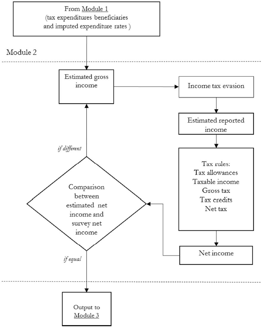
Net-to-gross conversion (Module 2).
For each taxpayer the procedure estimates an initial true gross income based on an average tax rate applied to net income as collected in the survey19, then applies an individual tax evasion rate, and then simulates the appropriate 2010 tax rules to produce a net income measure20, to be compared with the It-Silc one. If they differ, a new estimate of the true gross income is computed applying a correction factor, equal to the ratio between the original and the estimated net income, to the previous round true gross income and a new iteration is run. When equality between the two values is achieved (up to 1 euro of difference), the iteration ends and the data are sent to Module 3 for the reweighting procedure. The output for each individual, feeding into the following modules, includes true gross income, tax evasion rate, estimated reported income, deductions and tax credits, and gross and net income tax liability.
Table 4 below compares descriptive statistics for the components of gross income by income source obtained from our model with those available in It-Silc. It is interesting to observe, with respect to self-employment income, that Betamod produces a lower estimated gross income, reflecting our tax evasion modelling yielding higher tax evasion rates. Differences observed for other income sources are plausibly reflecting our reweighting procedure, illustrated in the following section, which aims at obtaining a representative sample of both population totals and the number of taxpayers.
Components of gross income: Betamod and It-Silc.
| Individuals | Households | |||||||
|---|---|---|---|---|---|---|---|---|
| Number of individualsa | Average gross incomeb | Number of householdsa | Average gross incomeb | |||||
| BETAMOD | IT-SILC | BETAMOD | IT-SILC | BETAMOD | IT-SILC | BETAMOD | IT-SILC | |
| Employment income | 21,179 | 21,382 | 20,229 | 20,110 | 15,133 | 14,887 | 29,237 | 28,884 |
| Pensions | 15,181 | 15,130 | 15,271 | 16,505 | 12,257 | 11,696 | 19,031 | 21,351 |
| Self-employment income | 6,728 | 6,882 | 21,876 | 22,095 | 5,955 | 5,762 | 26,098 | 26,384 |
-
Notes
-
a
thousands of persons
-
b
millions of euros
3.3 Reweighting module
Calibration weighting is a general technique for adjusting probability-sampling weights as of It-Silc so that model estimates are consistent with external official data sources (among others, see Atkinson et al., 1988; D’Amuri and Fiorio, 2006). As external data sources, we consider both population counts (from Istat official statistics) and official fiscal data (Mef).
While It-Silc weights are built to match population totals (Istat), we adjust them to achieve consistency with fiscal data as well, so that the model estimates are reconciled with both the entire population and taxpayers counts. The variables used for performing the individual level grossing- up are reported in Table 5. In addition to the standard socio-demographic variables, we also consider the number of taxpayers with dependent family members because of the important discrepancies between the sample distribution of household composition and official tax returns data. We obtain the joint distribution across those variables using the marginal distributions in a Ras-like iterative proportional fitting. The household weights are then computed by averaging individual household members weights21. As apparent in the last colum of Table 5, the achieved difference between Betamod recalibrated weights and external official data totals are appealing with respect to model estimates representativeness.
The grossing-up results.
| Variable | It-Silc weight | Official tax returns | Betamod weight | Difference |
|---|---|---|---|---|
| Total Population | 60,683,909 | - | 60,683,909 | 0 |
| Males | 29,499,829 | - | 29,499,827 | −2 |
| Females | 31,184,080 | - | 31,184,081 | 1 |
| North West | 16,131,196 | - | 16,131,196 | 0 |
| North East | 11,647,123 | - | 11,647,123 | 0 |
| Center | 11,943,354 | - | 11,943,354 | 0 |
| South | 20,962,237 | - | 20,962,237 | 0 |
| Age 0 – 14 | 8,841,850 | - | 8,841,850 | 0 |
| Age 15 – 24 | 6,041,469 | - | 6,041,468 | −1 |
| Age 25 – 44 | 17,172,717 | - | 17,172,717 | 0 |
| Age 45 – 64 | 16,394,019 | - | 16,394,019 | 0 |
| Age over 65 | 12,233,854 | - | 12,233,855 | 1 |
| Total households | 25,217,462 | - | 25,217,462 | 0 |
| North West | 7,186,593 | - | 7,186,593 | 0 |
| North East | 4,993,636 | - | 4,993,636 | 0 |
| Center | 5,007,637 | - | 5,007,637 | 0 |
| South | 8,029,596 | - | 8,029,596 | 0 |
| Total Taxpayers | - | 41,168,189 | 41,168,317 | 128 |
| Males | - | 21,622,165 | 21,622,249 | 84 |
| Females | - | 19,546,024 | 19,546,068 | 44 |
| North West | - | 11,653,491 | 11,653,533 | 42 |
| North East | - | 8,710,500 | 8,710,532 | 32 |
| Center | - | 8,317,613 | 8,317,638 | 25 |
| South | - | 12,486,585 | 12,486,613 | 28 |
| Reported income classes | ||||
| 1st quintile | - | 8,359,593 | 8,357,026 | −2,567 |
| 2nd quintile | - | 7,753,926 | 7,754,008 | 82 |
| 3rd quintile | - | 10,526,834 | 10,527,087 | 253 |
| 4th quintile | - | 7,851,917 | 7,852,371 | 454 |
| 5th quintile | - | 6,675,919 | 6,677,825 | 1,906 |
| Taxpayers by main income | ||||
| Employment income | - | 20,228,316 | 20,228,944 | 628 |
| Pensions | - | 14,165,864 | 14,166,862 | 998 |
| Self-employment income | - | 4,708,272 | 4,706,768 | −1,504 |
| Rental income from immovable property | - | 2,065,737 | 2,065,744 | 7 |
| Number of taxpayers with dependent family members | - | 12,624,414 | 12,624,454 | 40 |
3.4 The tax evasion module
According to the previous empirical literature concerning tax evasion at micro-level in Italy (Bernasconi & Marenzi, 1997; Florio & D’Amuri, 2006), we apply the “discrepancy method” to estimate tax evasion rates. The method, based on the assumption that individuals report a more truthful income to an anonymous interview than to fiscal authorities, computes tax evasion by comparing the tax returns and income survey responses of similar individuals.
In the above mentioned studies the comparison is made in terms of after-tax income. This choice has two main drawbacks. Firstly, it overestimate the tax evasion rates since it computes them as the ratio of evaded income on net income, instead of on true gross income. Secondly, when taxpayers are compared by quantiles of net incomes, a problem of re-ranking may arise. In fact, with respect to the distribution of after-tax income recorded in the survey, tax evasion shifts downwards individuals in the distribution of net income in the official data, so that, especially at low-income classes, the tax evasion rates are over-estimated. To overcome these drawbacks, Betamod estimates tax evasion rates as the percentage differences between the true gross incomes (as resulting from the net-to-gross conversion module) and the reported incomes declared to fiscal authorities. Clearly, since the true gross income is unknown and it is the results of the net-to gross procedure, tax evasion may be affected by approximations that depends on the estimation method.
Tax evasion rates are estimated in three steps (see Appendix B). In the first step, aggregate tax evasion rates, stratified by area and main income source type, are computed comparing simulated true gross incomes with administrative tax data on reported income. As administrative data are provided in aggregates, by main income source type and, separately, by geographical area, we first apply a Ras technique to obtain the joint distribution of reported income by both dimensions. As a result, a 4×4 matrix of average evasion rates, by income type and geographical area, is obtained (see Table 12).
In the second step a distributional income profile of tax evasion is estimated for each area-by- income type stratum. We refine stratification expanding the 16 strata to account for the profile of tax evasion by income classes. In more detail, each area-by-income type stratum is expanded into 13 classes of true gross income, so that 16 income profiles of tax evasion are obtained. The design of each evasion-by-income profile results from an optimizing procedure, which aims at minimizing the distance between simulated and administrative reported income. The result is a 16×13 dimension matrix of tax evasion rates by main income source type, geographical area and true gross income level.
Finally, a tax evasion rate is assigned to each individual for each type of income source to overcome the standard procedure of assigning the same tax evasion rate to all individuals in each matrix cell. Betamod selects randomly, within each cell, individuals to be identified as tax compliers, and those to be identified as tax evaders, then assigns individual tax evasion rates by using a beta distribution whose mean value is equal to the average tax evasion rate of the cell. Namely, individual tax evasion rates are calibrated so that the sum of individual evaded incomes is equal to the total income evaded in the class. This represents an advancement, with respect to other models, where tax evasion rates are assumed to be constant within population subgroups (e.g. by income source type, by income classes). This feature allows assessing the relevance of re-ranking between tax-payers due to the presence of tax evasion.
4. Validation and main results
The ability of Betamod to reproduce each measure (gross income, taxable income, deductions, tax credits and net tax liability) relevant for personal income tax and local income taxes is validated through a comparison with official figures provided by tax returns data for the relevant fiscal year, that is 2010. To do this, we first compare the aggregate tax figures simulated by Betamod with the official fiscal statistics. Results are shown in Tables 6, 7 and 8.
Aggregate validation: main components of personal income tax and local taxes.
| Number of taxpayersa | Valueb | |||||
|---|---|---|---|---|---|---|
| Totals | Betamod | Official tax returns | Diff. % | Betamod | Value ² Official tax returns | Diff. % |
| Gross income | 41,168 | - | - | 853,891 | - | - |
| Evaded income | 14,778 | - | - | 60,789 | - | - |
| Reported income | 41,168 | 41,168 | 0.0 | 793,102 | 792,520 | 0.1 |
| Deductions | 13,794 | 13,374 | 3.1 | 21,736 | 21,746 | 0.0 |
| Taxable income | 41,097 | 39,894 | 3.0 | 763,086 | 762,185 | 0.1 |
| Gross tax liability | 41,097 | 39,078 | 5.2 | 205,213 | 205,613 | −0.2 |
| Tax credits | 39,977 | 39,088 | 2.3 | 64,604 | 62,482 | 3.4 |
| Net tax liability | 31,178 | 30,897 | 0.9 | 147,904 | 149,443 | −1.0 |
| Regional income tax | 31,035 | 30,653 | 1.2 | 8,655 | 8,633 | 0.3 |
| Municipal income tax | 25,251 | 25,265 | −0.1 | 3,023 | 3,021 | 0.1 |
-
Notes
-
a
thousands of persons
-
b
millions of euros
Aggregate validation: deductions.
| Number of taxpayersa | Valueb | |||||
|---|---|---|---|---|---|---|
| Deductions | Betamod | Official tax returns | Diff. % | Betamod | Value ² Official tax returns | Diff. % |
| Social insurance contributions paid by self-employed individuals | 11,922 | 11,991 | −0.6 | 17,601 | 17,603 | 0.0 |
| Cadastral value of the main residence | 16,873 | 17,166 | −1.7 | 8,279 | 8,283 | 0.0 |
| Voluntary contributions to private pension plans | 803 | 822 | −2.3 | 1,897 | 1,905 | −0.4 |
| Legal alimony payments for spouse | 109 | 120 | −9.5 | 742 | 745 | −0.4 |
| Personal care services and disability aids | 147 | 143 | 2.8 | 537 | 531 | 1.2 |
| Social insurance contributions paid for domestic help | 522 | 537 | −2.8 | 415 | 419 | −0.9 |
| Donations to religious institutions | 95 | 104 | −8.7 | 27 | 27 | −1.8 |
| Others | 1,800 | 1,816 | −0.9 | 517 | 516 | 0.1 |
-
Notes
-
a
thousands of persons
-
b
millions of euros
Aggregate validation: tax credits.
| Number of taxpayersa | Valueb | |||||
|---|---|---|---|---|---|---|
| Deductions | Betamod | Official tax returns | Diff. % | Betamod | Value ² Official tax returns | Diff. % |
| Income source tax credit | 37,852 | 36,426 | 3.9 | 44,475 | 41,887 | 6.2 |
| Dependent family members tax credit | 12,624 | 12,624 | 0.0 | 10,914 | 11,375 | −4.0 |
| 19% tax credits | ||||||
| Healthcare expenses | 14,855 | 15,002 | −1.0 | 2,588 | 2,585 | 0.1 |
| Mortgage interest payments on main residence | 3,817 | 3,841 | −0.6 | 1,146 | 1,147 | 0.0 |
| Life insurance premium 6,437 | 6,520 | −1.3 | 750 | 751 | −0.1 | |
| Secondary and tertiary education | 2,102 | 2,095 | 0.3 | 318 | 318 | 0.0 |
| Funeral expenses | 413 | 428 | −3.6 | 119 | 119 | −0.4 |
| Mortgage interest payments on other properties | 281 | 296 | −5.1 | 80 | 77 | 3.2 |
| Annual enrollment to sports facilities | 1,506 | 1,522 | −1.1 | 60 | 60 | 0.1 |
| Rent for resident students | 159 | 169 | −6.2 | 51 | 50 | 1.0 |
| Social/community/home care expenses | 113 | 108 | 4.0 | 38 | 38 | 0.6 |
| Charitable donations | 899 | 915 | −1.8 | 36 | 36 | 0.3 |
| Real estate brokerage expenses | 95 | 100 | −4.1 | 16 | 15 | 1.5 |
| Others | 1,080 | 1,101 | −1.9 | 83 | 83 | −0.1 |
| 55% tax credits | ||||||
| For energy conservation's interventions | 1,038 | 1,052 | −1.4 | 1,351 | 1,349 | 0.1 |
| 41%-36% tax credits | ||||||
| House refurbishments | 5,175 | 5,267 | −1.8 | 2,242 | 2,243 | 0.0 |
| 20% tax credit | 539 | 540 | −0.1 | 65 | 65 | −0.1 |
| Others tax credits | ||||||
| For tenants subject to controlled rent and for employees relocating closer to work | 708 | 713 | −0.7 | 138 | 136 | 1.5 |
| Security sector tax credit | 375 | 349 | 7.5 | 50 | 50 | 0.0 |
| Others | 158 | 137 | 15.3 | 84 | 83 | 1.6 |
-
Notes
-
a
thousands of persons
-
b
millions of euros
First, it should be noted that tax evasion reduces the true gross income of about 61 billions of euro, corresponding to an average tax evasion rate of 7.2 per cent. The estimated tax evasion rate might seem relatively low in a country, like Italy, where tax evasion is a widespread phenomenon (among others, Marino and Zizza, 2012; Fiorio and D’Amuri, 2006). However, the figure reflects the fact that employment income and pensions taken as a whole account for more than the 80% of total reported income (53% and 29%, respectively) and that the estimated average tax evasion rates for these two types of income are, respectively, 2.9 per cent and zero. As apparent in Table 6, Betamod output and official fiscal data presents trivial (i.e. lower than 1%) differences in most figures achieving a very good performance in simulating revenues amounts and taxpayers’ counts22.
The largest difference arises in the number of individuals with positive gross tax liability. This seems mostly driven by the model imputation of tax deductions, resulting in a larger number of individuals with positive taxable income in Betamod. This is because tax deductions have been imputed as a percentage of reported income, thus constraining their amount to be lower than reported income, and therefore taxable income to be positive, by construction. In addition, tax rules require some taxpayers to report a zero gross tax liability even if it is in fact positive: this applies for example to pensioners with gross income (excluding the cadastral return on main residence) lower than 7,5 thousands euros, or to taxpayers whose only income, if lower than 500 euros, is that from buildings.
Focussing on deductions, Table 7 reports the number and the amount of beneficiaries for each type. Again, no significant differences are found between Betamod results and tax returns data, in particular, Betamod replicates well the largest deduction (the social insurance contributions).
Some discrepancies can be observed only in simulating the number of deduction beneficiaries for donations to religious institutions (-8.7%) and for alimony payments to the spouse (-9.5%). In both cases the number of tax relief claimants is anyway negligible. Table 8 considers tax credits, covering both the model-simulated and the imputed ones. In general, Betamod estimates provide a good approximation of the tax returns figures.
The number of beneficiaries and the amount of the income-source tax credit are overestimated of about 3.9% and 6.2% respectively. This is mainly due to the fact that estimated reported incomes are more dense in the bottom of the distribution in Betamod than in tax data. Since the tax credit is decreasing in income, the Betamod tax credit results greater than in tax returns data. As to the dependent family members tax credit, the striking similarity in the number of beneficiaries is motivated by this variable having been taken into account in the weighting design, while the simulated amount of tax credit is -4.0% lower than the official figure, presumably reflecting the sample distribution of household composition, relevant for identification of dependants. The other most sizeable tax credits, namely healthcare expenditures, house refurbishment, energy interventions and mortgage interest tax credits are remarkably close to the administrative figures. As expected, the main discrepancies arise in the numbers of beneficiaries of the less sizeable tax credits23.
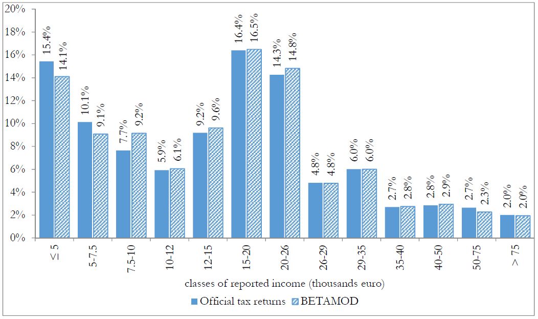
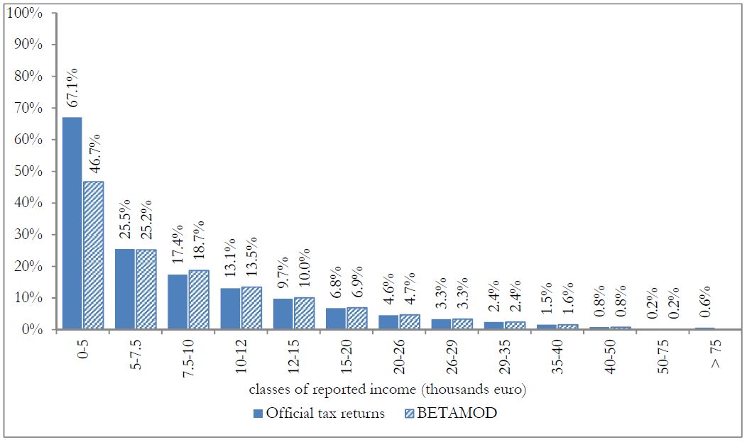
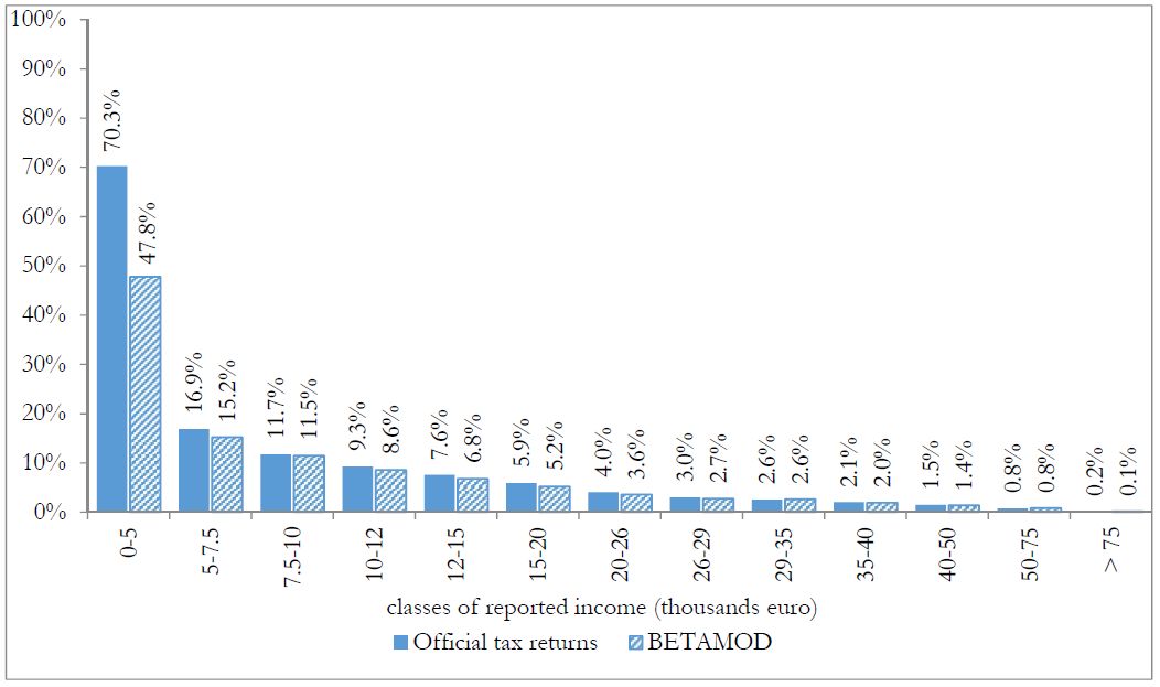
Besides assessing the model validity at the aggregate level, no less attention should be devoted to the validation of the distributional patterns of different components of the model output, as it mainly represents a tool for carrying out distributional analyses. First, we compare the distribution of taxpayers (Figure 3) and of simulated reported income (Figure 4) with official statistics. Overall, the Betamod distributions are strikingly similar to the fiscal data ones, especially in the classes of reported income where most of taxpayers fall (12–26 thousands of euros). Such pattern of similarity is confirmed when considering the distribution of average gross and net tax liabilities across income classes (Table 9). The following Figures 5 and 6 represent the progressive design of the income source and the family dependents tax credits, as arising from Betamod and from tax returns data. Again, the similarity between the two is striking, and is also confirmed for other tax allowances (the related figures are reported in Appendix C). Interestingly, both tax credits are partly lost by taxpayers in the bottom income class, due to their low level of taxable income/gross tax liability, and to the non-refundable nature of these tax credits.

Distribution of taxpayers by classes of reported income.

Distribution of reported income by classes of reported income.

Income source tax credit as a proportion of reported income (%).
Tax credit for dependent family members as a proportion of reported income.
Gross and net tax distribution by classes of reported income (mean values in euros).
| Classes of reported income | Gross tax liability | Net tax liability | ||
|---|---|---|---|---|
| Betamod | Official tax returns | Betamod | Official tax returns | |
| under 5,000 | 442 | 453 | 281 | 229 |
| 5,000 – 7,500 | 1,317 | 1,394 | 613 | 460 |
| 7,500 – 10,000 | 1,851 | 1,938 | 415 | 492 |
| 10,000 – 12,000 | 2,437 | 2,417 | 826 | 867 |
| 12,000 – 15,000 | 2,998 | 2,993 | 1,384 | 1,426 |
| 15,000 – 20,000 | 4,005 | 3,988 | 2,373 | 2,336 |
| 20,000 – 26,000 | 5,363 | 5,359 | 3,745 | 3,673 |
| 26,000 – 29,000 | 6,612 | 6,584 | 5,026 | 4,952 |
| 29,000 – 35,000 | 7,979 | 7,966 | 6,403 | 6,401 |
| 35,000 – 40,000 | 10,077 | 9,962 | 8,763 | 8,513 |
| 40,000 – 50,000 | 12,634 | 12,439 | 11,452 | 11,169 |
| 50,000 – 75,000 | 18,111 | 18,244 | 17,134 | 17,228 |
| above 75,000 | 45,707 | 46,799 | 44,166 | 45,551 |
| Average | 4,993 | 5,262 | 4,744 | 4,837 |
Although comparison with other Italian microsimulation studies (e.g. Fiorio and D’Amuri, 2005; Tomarelli and Acciari, 2010; Di Nicola et al., 2015) is hindered by differences in the fiscal years considered, as well as by different modelling choices, the redistributive impact and progressivity design estimated by Betamod result broadly in line with those.
Further insight into the distributional effect of different personal income tax components, can be gained decomposing the overall progressivity impact, as measured by the Kakwani index shown in Table 10. This reflects both the tax design (i.e. provisions for tax exemptions, deductions, the tax rate schedule, tax credits) and the effect of tax evasion. We build on a reinterpretation of the Pfähler (1990) decomposition of Kakwani index25, in the spirit of Verbist and Figari (2013). In more detail, the total Kakwani progressivity index πkTpit can be expressed as a weighted sum26 of gross tax liability progressivity πkK and tax credits progressivity πkK, as in:
Inequality and redistributive indices.
| Individuals | Equivalent households | |||
|---|---|---|---|---|
| Gini | Concentration | Gini | Concentration | |
| Gross income | 0.4155 | 0.4155 | 0.3885 | 0.3885 |
| Reported income | 0.4417 | 0.4264 | 0.4060 | 0.3954 |
| Taxable income | 0.4478 | 0.4262 | 0.4102 | 0.3950 |
| Gross tax liability | 0.5107 | 0.4909 | 0.4702 | 0.4552 |
| Net tax liability | 0.6784 | 0.6508 | 0.6315 | 0.6104 |
| Net income | 0.3678 | 0.3662 | 0.3428 | 0.3415 |
| Reynolds-Smolensky index | 0.0493 | 0.0469 | ||
| Kakwani index | 0.2353 | 0.2220 | ||
| Average tax rate | 0.1732 | 0.1745 | ||
| Reranking effect | 0.0015 | 0.0013 | ||
In other words, the progressivity of gross tax liabilities (πkTg) is further decomposed in a direct progressivity effect resulting from the tax rate schedule πkR and an indirect progressivity effect depending on the amounts of various exemptions/deductions πkE πkD from gross income. Our decomposition measures directly also the contribution to progressivity of tax evasion πkEV. Each Kakwani index show the degree of disproportionality in each tax component, relative to the distribution of gross income. Results are shown in Table 11, with Kakwani indices reported in the last column.
Kakwani indices of Personal Income Tax components.
| Equivalent households | ||||||
|---|---|---|---|---|---|---|
| Average rate of tax components | Weight of the decomposition | Kakwani index | ||||
| Evasion | ev | 0.0686 | ev/(1-ev-e-d) | 0.0765 | πkEV | 0.0945 |
| Exemptions | e | 0.0104 | e/(1-ev-e-d) | 0.0116 | πkE | 0.0389 |
| Deductions | d | 0.0245 | d/(1-ev-e-d) | 0.0273 | πkD | −0.0393 |
| Tax rate schedule | πkR | 0.0602 | ||||
| Gross tax liability | tg | 0.2408 | tg/tn | 1.3797 | πkTg | 0.0668 |
| Tax credits | k | 0.0663 | k/tn | 0.3797 | πkK | 0.3419 |
| Tax credits for income source | kis | 0.0486 | kis/tn | 0.2782 | πkKis | 0.3989 |
| Tax credits for dependent family members | kdf | 0.0077 | kdf/tn | 0.0444 | πkKdf | 0.5329 |
| k19 | 0.0056 | k19/tn | 0.0323 | πkK19 | −0.0196 | |
| 19% tax credits | ko | 0.0043 | ko/tn | 0.0249 | πkKo | −0.1684 |
| Other tax credits | tn | 0.1745 | tn/(1-tn) | 0.2115 | πkTn | 0.2220 |
| Net tax liability | ev | 0.0686 | ev/(1-ev-e-d) | 0.0765 | πkEV | 0.0945 |
Tax evasion and exemptions (namely the cadastral value of the main residence) enhance progressivity, whereas deductions are wholly regressive. The effect of tax evasion is mainly due to its negative income gradient, reducing gross income more at the lower end of the distribution. The exemption of imputed rent increases progressivity since this figurative income component is proportionally more sizeable for lower income taxpayers. On the other hand, deductions have an inequality enhancing impact, plausibly motivated by the proportional effect of social insurance contributions on the self-employed being offset by pro-rich pattern of personal expenses. Not surprisingly, the tax schedule exhibits a major progressivity effect. It is tax credits though that are the most important determinant of progressivity, their contribution amounting to about 58% of overall progressivity. This is mostly driven by income-source and dependent family members tax credits, whose design entails positive withdrawal rates as taxable income increases. Other tax credits, subsidizing personal spending on a wide range of goods and services, including housing, healthcare and education, while less sizeable, do display a regressive effect.
Clearly, the overall progressivity impact of each component depends on their relevance with respect to gross income. For instance, the value of the Kakwani index for the dependent family members tax credit is remarkably higher (0.5329) than the one for the income-source tax credits (0.3989), but the contribution to progressivity of the latter exceeds that of the former because of the relative weights.
5. Tax evasion and its distributional profile
To showcase Betamod potential for analysis, in this section we provide some distributional evidence on tax evasion. According to our estimates, on aggregate €61 billions of gross income escape tax authorities, corresponding to a tax revenue loss amounting to about €16 billions27. Unsurprisingly, tax evasion arises mostly from self-employed income and, to a lesser extent, rental income from property: overall, 85% of evaded income is attributable to these two sources (65% and 20% respectively). The remaining 15% of evaded income is attributable to employment income, as pension income, representing a public transfer, can hardly be hidden from tax authorities.
Average tax evasion rates, by income source and geographical area, are reported in Table 12. The figures reveal that tax evasion on employment income, while not negligible, is low (2.9%), and that the largest tax evasion rates are registered on rental income from immovable property (33.6%) and self-employment income (24%). Relevant differences arise also between geographical areas: in particular, our results identify individuals living in the South of Italy as those displaying systematically higher tax evasion rate, followed by those in the North East. The Betamod estimated average values are slightly lower, yet not inconsistent, with estimates derived by above mentioned studies on tax evasion in Italy.
Average tax evasion rates by income source and geographical area (%).
| Average tax evasion rate | NW | NE | C | S | ITALY |
|---|---|---|---|---|---|
| Employment income | 2.7 | 3.1 | 2.8 | 3.3 | 2.9 |
| Pensions | 0.0 | 0.0 | 0.0 | 0.0 | 0.0 |
| Self-employment income | 22.2 | 25.1 | 22.3 | 27.2 | 24.0 |
| Rental income from immovable property | 30.6 | 35.5 | 31.3 | 38.2 | 33.6 |
| Total income | 6.9 | 7.5 | 6.8 | 7.7 | 7.2 |
As arises from Figure 7 (a,b,c), the distribution of tax evasion rates varies across different income sources. Among individuals who hide employment income from tax authorities, low tax evasion rates are most often estimated. On the contrary, more than half of self-employed income tax evaders display a tax evasion rate that is higher than 60%. A similar distribution arises for rental income evasion; about 50% of rental income tax evaders display tax evasion rates between 60 and 80%. Figure 7d plots the full distribution of estimated individual tax evasion rates, by true gross income, i.e. the ‘true’ amount individuals would report to tax authorities under full compliance. The Figure reveals that individuals’ tax evasion rates cluster around an upper and a lower level, reflecting the underlying individual income sources composition, i.e. the prevalence of employment (relatively low level of tax evasion) versus self-employed and rental incomes (high level of tax evasion). The evidently negative gross income gradient of tax evasion rates clearly reflects the tax evasion estimation procedure, which accounts for evasion-by-income profiles28.
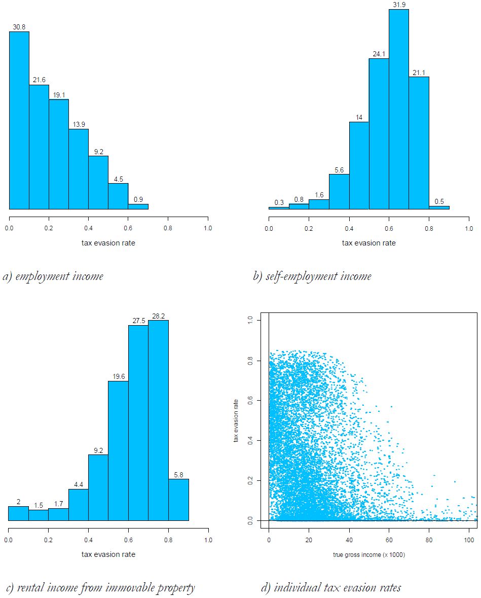

Distribution of tax evasion rates by type of income (tax evaders only, in percentage).
The following Figure 8, where tax evasion rates by income class are shown, provides further evidence on the negative gross income gradient of tax evasion rates, and allows to better gauge the income profile of tax evasion behaviour by income source as well. In relative terms, both for each income source, and for their aggregate, consistently with previous studies (Bernasconi & Marenzi, 1997; Fiorio & D’Amuri, 2006), Betamod reflects tax evasion rates generally decreasing in income29. With respect to those works, Betamod yields a flatter income gradient for tax evasion by employees in the lower income classes. This plausibly comes as a consequence of our tax evasion rate being computed over gross income, while their figures are based on net incomes at the denominator.
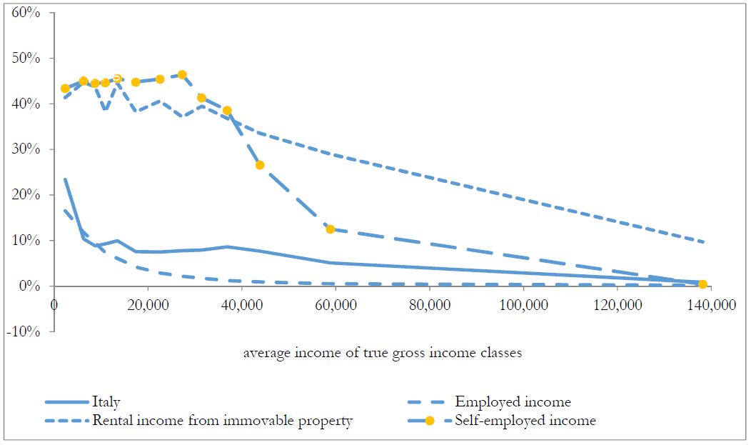

Average tax evasion rates by type of income and by true gross income classes.
Figure 9 shows the total amount of unreported income. It can be noticed that, despite the decreasing profile of tax evasion rates, most of evaded income is due to taxpayers with gross income in the range 12,000–50,000 euro, and mainly to self-employed income.
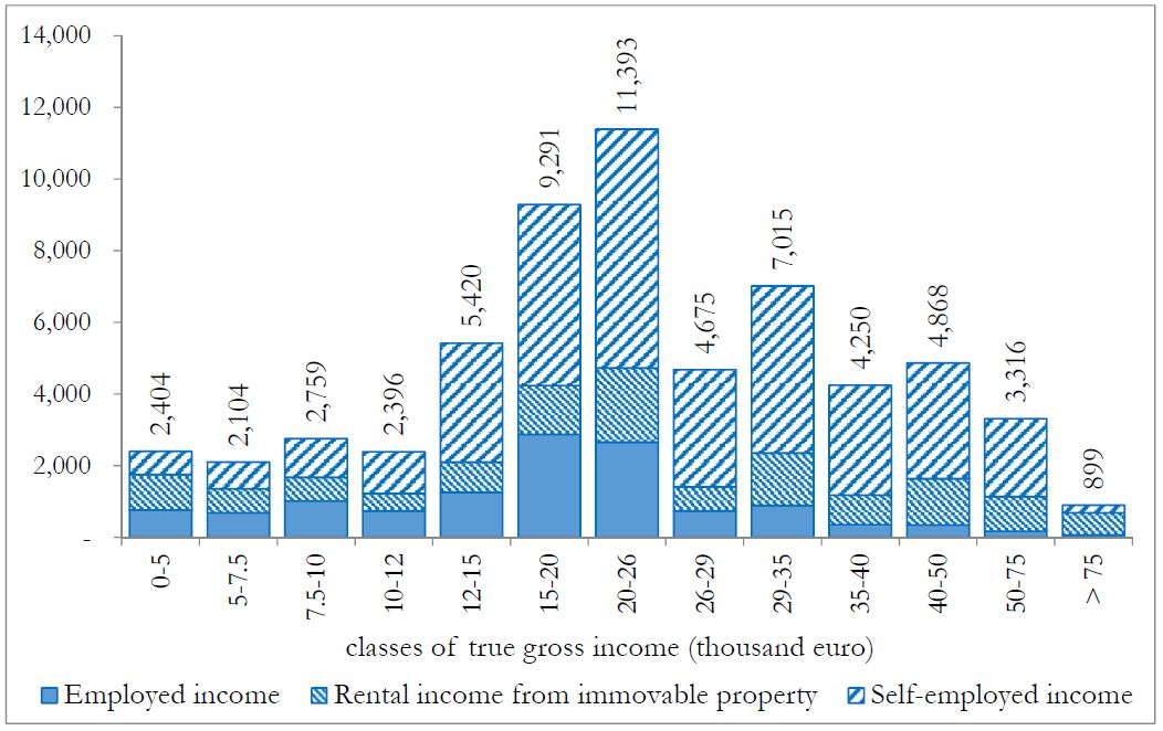

Unreported income by classes of true gross income (millions of euros).
Tax evasion, by reducing reported income, causes a relevant downward shift in the distribution of taxpayers by reported income, with respect to that by (true) gross income. To begin with, tax evasion may modify the relative position (in terms of reported income) between fully-compliant taxpayers and same-true-gross-income evaders, generating an horizontal inequity effect in income taxation. Indeed, while horizontal inequity is one of the major consequence of tax evasion, very little studies measuring it exist. Betamod evidence is provided in Figure 10, where the two cumulative distributions of taxpayers, by (true) gross and reported income respectively, are shown. The distribution of individuals by reported income is thicker in the left tail, when compared with the distribution of gross income, suggesting a downward movement, along the income distribution, of taxpayers who “benefit” from tax evasion.
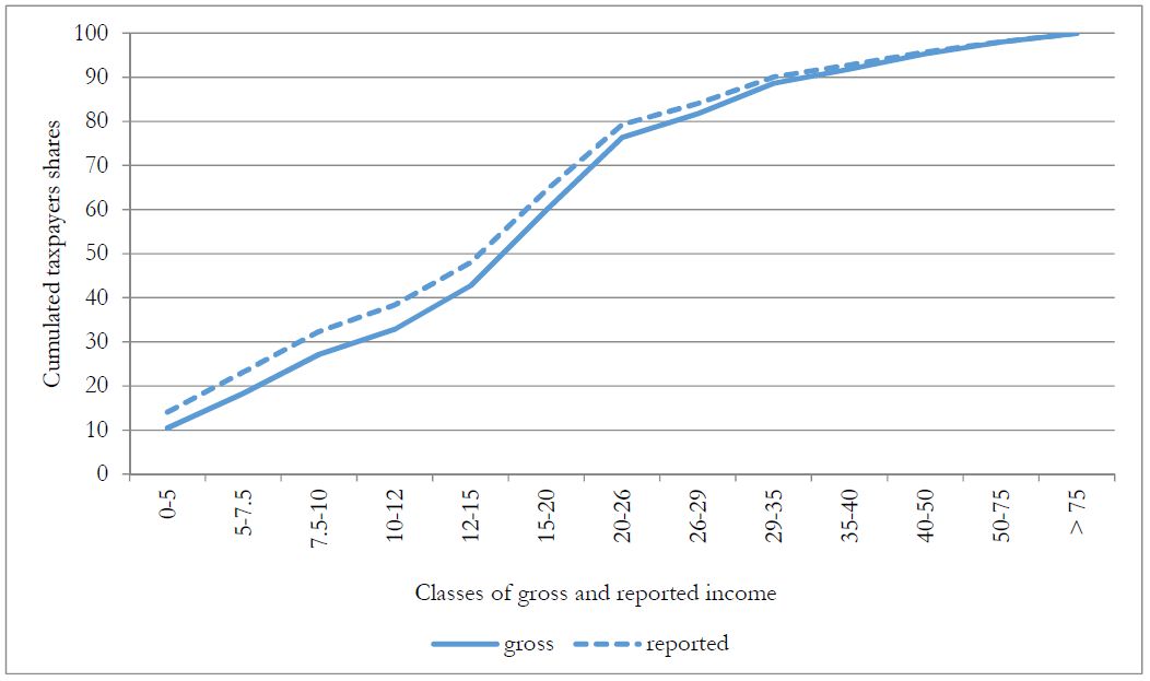
Cumulative distributions of taxpayers by (true) gross and reported income classes (thousands of euros).
Betamod transition matrix, reporting the share of true gross income taxpayers falling in each income class, found in different reported income classes as a result of tax evasion, is reported in Table 13. As a result of non-compliance, the taxpayers in the bottom income class, for instance, moves from about 10% when considering true gross income to about 14% when considering reported income relevant for taxation. Evaders who enter the bottom income class come from the 2nd to the 8th income class (up to 29 thousands of euros), rather than from higher income classes, reflecting the decreasing income profile of tax evasion rates. Moving to the upper classes, we observe a similar pattern of shifts across income classes, although the number of shifts is progressively reduced, again because of the negative income gradient in tax evasion. While Table 10 only reports between class shifts, building on the availability of individual tax evasion rates, Betamod allows to detect further shifts happening within each income class.
Transition matrix of taxpayers from (true) gross income to reported income (%).
| Classes of true gross income (thousands of euros) | |||||||||||||||
| 0–5 | 5–7.5 | 7.5–10 | 10–12 | 12–15 | 15–20 | 20–26 | 26–29 | 29–35 | 35–40 | 45–50 | 50–75 | >75 | Total | ||
| Classes of reported income (thousands of euros) | 0–5 | 10.47 | 1.51 | 0.79 | 0.33 | 0.57 | 0.33 | 0.11 | 0.01 | 14.11 | |||||
| 5–7.5 | 6.37 | 0.91 | 0.43 | 0.42 | 0.52 | 0.32 | 0.07 | 0.04 | 9.08 | ||||||
| 7.5–10 | 7.13 | 0.60 | 0.49 | 0.34 | 0.39 | 0.11 | 0.08 | 0.02 | 9.15 | ||||||
| 10–12 | 4.38 | 0.71 | 0.50 | 0.25 | 0.06 | 0.11 | 0.04 | 0.01 | 6.06 | ||||||
| 12–15 | 7.66 | 1.25 | 0.31 | 0.08 | 0.17 | 0.09 | 0.04 | 9.61 | |||||||
| 15–20 | 14.26 | 1.64 | 0.24 | 0.19 | 0.09 | 0.05 | 16.50 | ||||||||
| 20–26 | 13.43 | 0.72 | 0.43 | 0.12 | 0.11 | 0.01 | 14.82 | ||||||||
| 26–29 | 4.06 | 0.51 | 0.12 | 0.08 | 0.01 | 4.78 | |||||||||
| 29–35 | 5.34 | 0.37 | 0.23 | 0.06 | 6.01 | ||||||||||
| 35–40 | 2.38 | 0.31 | 0.05 | 2.75 | |||||||||||
| 40–50 | 2.64 | 0.30 | 2.94 | ||||||||||||
| 50–75 | 2.25 | 0.02 | 2.26 | ||||||||||||
| > 75 | 1.95 | 1.95 | |||||||||||||
| Total | 10.47 | 7.88 | 8.83 | 5.74 | 9.85 | 17.21 | 16.45 | 5.36 | 6.86 | 3.23 | 3.48 | 2.67 | 1.96 | 100 | |
Once taxation applies to reported income, shifts along the income distribution, give rise not only to horizontal inequities, but also to a re-ranking effect, with a reversal of taxpayers’ relative positions before (i.e. reflecting the true gross income position) and after personal income taxation (i.e. based on the reported income position ), which the model also allows studying. Although preliminary, the novel empirical evidence showcased here bears major implications for the accurate measurement of the actual redistributive effect of personal income taxation and its decomposition in the horizontal, vertical and re-ranking effect, each of which is possibly altered by tax evasion.
Footnotes
1.
In the past decade several microsimulation models were developed in Italy. For instance: the Siena microsimulation model (SM2) for net-gross conversion of Eu-Silc income variables (Betti et al. 2011); the Mapp model for studying the effects of taxes and transfers (in cash and in kind) on the level of poverty and inequality (Baldini et al., 2011); the Tabeita model that reproduces the Italian personal income tax (Ceriani et al., 2013), and the microsimulation model developed by Pellegrino et al. (2011) for the analysis of housing taxation.
2.
Further material is provided in three Appendices. Appendix A describes the statistical matching between the It-Silc dataset and the Bank of Italy’s Survey on Households Income and Wealth (Shiw); Appendix B illustrates the methodology used for the estimation of individual tax evasion rates, and Appendix C shows the incidence of tax reliefs on reported income.
3.
For instance, SM2 model (Betti et al., 2011), Mapp model (Baldini et al., 2011), and the Euromod module for Italy (Sutherland and Figari, 2011) use It-Silc data; while, Tabeita model (Ceriani et al., 2013) and the microsimulation model developed by Pellegrino et al. (2011) considers as input data those provided by the Bank of Italy in the Survey on Households Income and Wealth (Shiw).
4.
Non-taxable incomes and benefits are taken from the survey, rather than simulated, in order to obtain the disposable income measure.
5.
While cadastral income on the main residence is de facto exempted from personal income taxation trough a tax deduction, it is anyway relevant for other components of the tax benefit system, such as the means test for family benefits. For other properties, according to whether they are rented or left unoccupied, the actual rent received or cadastral income are respectively used in tax base assessment.
6.
The Shiw question asks respondents to assess subjectively the value of each of their properties.
7.
The Ras algorithm is an iterative proportional fitting procedure that estimates joint distribution of two or more variables given their marginal distributions. See Bacharach (1965).
8.
More precisely, the ratio has been multiplied by a 1.05 correction factor, to reflect a legislated uprating adjustment.
9.
When secondary properties are rented, the actual rent received, as collected in It-Silc, rather than cadastral income, enters in the tax base definition.
10.
The Multiscopo Survey did not take place in 2010. Even though time distance between the interviews in It-Silc 2010 and Multiscopo Survey 2013 seems quite large, this does not constitute an issue since we only used qualitative information that are actually comparable between the two datasets.
11.
We have not included income among the control variables since the Multiscopo Survey does not provide any information about it. However, research findings have suggested that, while at aggregate level there exists a positive and significant relationship between healthcare expenditure and Gdp (Newhouse, 1977), at individual level, there is not a significant association between healthcare expenditure and income (especially when the health system provides universal coverage free of charge as the Italian healthcare system does). Indeed, full insurance coverage would remove the individual budget constraint and reduce or eliminate the influence of cost of care on patients’ decisions of how much care to use. Typically, income elasticity of individual healthcare expenditure under full insurance coverage regime tends to be near zero (for details see Getzen, 2000).
12.
We consider as self-employed members of the arts and or professions, sole proprietors, free lances, owners or members of a family business and persons receiving profits from non- corporate enterprises.
13.
By ‘reported incomes as estimated by the model’ we mean the portion of true gross income that we estimate the individual will declare, given his tax evasion rate. In what follows, this will be referred to as ‘estimated reported income’, as opposed to ‘reported income’, which refers to official tax returns data.
14.
The tax returns of the entire population of taxpayers are disposable on the website of the Italian Revenue Agency (Ministry of Economy and Finance) only in tabulated form (e.g. by type of income source, by income classes, by area of residence, etc.). Additional ad-hoc data were required for better modelling tax reliefs.
15.
The gross income qualified for tax reliefs is net of cadastral income on the main residence.
16.
Employees’ social contributions are not listed among deductions as they are excluded from taxable employment income.
17.
The simulation of tax credit for dependents required the construction of fiscal family that may not coincide with the definition of household adopted in It-Silc. In fact, fiscal family members include the spouse, children and other relatives living with the referent person and having a personal gross income (before deductions) below € 2,840.
18.
A notable exception is the Siena microsimulation model (SM2) which, building on an exact record linkage between survey and fiscal administration data (Consolini et al., 2006, Consolini et al., 2009, Donatiello et al., 2009), is able to account for the full set of tax expenditures as observed from fiscal data.
19.
The measurement of net labour earnings accounts for specific pay components, namely: net salary and additional compensations including the thirteenth/fourteenth monthly pay (a peculiarity of the Italian institutional setting), income from temporary project-based employment contracts, which are fiscally equivalent to employment income, and taxable unemployment benefits.
20.
In computing individual tax liabilities, deductions are subtracted from reported income, to obtain taxable income. The gross tax is calculated applying the tax schedule to taxable income. Then net tax is obtained subtracting tax credits from gross tax.
21.
An appropriate factor of correction is applied to ensure representativeness of households by geographical area.
22.
The regional income tax is simulated by Betamod while the municipal income tax is imputed.
23.
Simulating the correct number of beneficiaries in the quantitatively less important tax credits is, in fact, one of the most common challenges in microsimulation modelling due to the lack of information relevant for identification of potential claimants in the survey data, as well as to the small number of individuals involved.
24.
The household equivalent income is obtained by applying the OECD-modified equivalence scales. We compute household’s net income by adding all true gross income earned by the family members ad subtracting the personal tax liabilities.
25.
Kakwani index measures the departure from proportionality as the difference between the concentration coefficient of tax and the Gini index of gross income.
26.
The weight for the gross tax liability progressivity (πk ) is the ratio between gross tax rate (tg) and net tax rate (tn); the weight for tax credits progressivity (πkK) is the ratio between tax credits as a proportion of gross income (k) and net tax rate (tn).
27.
The tax revenue loss refers to the personal income tax (15 billions), regional and municipal additional income taxes (800 and 160 millions respectively).
28.
As previously explained in Section 3.4, the decreasing aggregate profile results by the comparison between Betamod simulated gross income and reported income to tax authorities.
29.
Results must be considered taking into account that they are based on the income distribution which directly emerges from It-Silc survey. However, the survey doesn’t guarantee representation of true income distribution. Previous studies, although based on Bank of Italy’s survey (e.g. Cannari and D’Alessio, 1992) have in particular identified two major biases, which are indeed common to surveys conducted in other countries. The first is the selectivity bias due to the fact that not all families are equally available to participate to the survey; the second is known as under-reporting, and arises when the respondent reports a disposable income below the true income. Both selectivity bias and under-reporting can explained with the fear that some people have that their files could be accessed by the tax authorities. Evidence indicates that the fear is more pronounced in individuals belonging to the upper tail of the distribution. A third, though less relevant, bias is originated by some over-reporting of people belonging in the lower tail. Clearly all three biases contribute to making the sample distribution less unequal than the real distribution.
A. Statistical matching between the IT-SILC and SHIW datasets
We describe here how the statistical matching between the IT-SILC dataset with the Bank of Italy's Survey on Households Income and Wealth (SHIW) at the household level was performed. First, two constraints need be satisfied to make matching feasible: (i) the two surveys must be random samples from the same population; (ii) there must be a common set of conditioning variables. In our case, the first condition is met by design, since both the IT-SILC 2011 and the SHIW 2012 data are representative of the Italian population. As far as the second constraint is concerned, the variables (X) common to each dataset and chosen for the process of imputation of self-reported asset value of the main residence, insurance premiums and house refurbishments expenditures are: equivalent household income, the percentage of household members with more than upper secondary educational qualification, a set of household composition dummies, and the main earner’s employment status. The final sample is made up of 7.951 households from the SHIW survey and 19.399 households from the IT-SILC Survey.
The dataset, integrated by IT-SILC-Bank of Italy was created using the Mahalanobis Distance Matching Method (MDMM), a statistical method which allows individuals with similar characteristics but from different datasets to be paired (Rosenbaum & Rubin, 1983). In order to obtain a more precise matching, the sample was stratified in cells according to the main residence homeownership, other properties homeownership and geographical area so that exact matching on these variables is ensured; then, within each stratum, the donor household has been selected based on the Mahalanobis distance metric, measured on the other X variables. The Mahalanobis metric is a measure of dissimilarity between observation which measures the distance between units i from the recipient dataset IT-SILC and j from the donor dataset SHIW weighting each coordinate of X in inverse proportion to the variance of that coordinate:
Matching has been performed at the household level and with replacement, that is allowing the same SHIW household to act as donor for multiple It-Silc households, if deemed as the most adequate, rather than being discarded after having served once as donor. Once the matching procedure was complete, we check the quality of the matching. The quality of matching was evaluated in terms of maintaining the asset value of the main residence, insurance premiums and house refurbishments expenditures distributions, both in terms of preserving the pre-existing variables distribution as well as in terms of pre-existing relations between variables of interest.
The next step was i) the comparison between the asset value of the main residence, insurance premiums and house refurbishments expenditures distributions in the integrated dataset and the pre-existing SHIW one, ii) the calculation of the correlation between asset value of the main residence, insurance premiums and house refurbishments expenditures distributions and the X vector to verify the maintenance of the sign recorded in the "donor set". The differences between the common-fusion correlations in the Shiw data set versus the fused It-Silc data set were well preserved for most variables. For the sake of brevity, tables showing distributions and correlations are not included but they are available on request.
Finally, the quality of the matching has been evaluated in terms of “balancing test”: we compared the mean covariate values in the recipients and matched donors i.e. each of the observable covariates within the recipients has the same average value within the matched donors. Before matching we expect differences, after matching the variables should be balanced in both groups and significant differences should not persist. The covariate balancing test, included in Table A1, shows that the matching is effective in removing differences in observable characteristics between the recipients and matched donors. In particular, the median absolute bias is reduced by approximately 82%-98%. The Pseudo R-squared after matching is always close to zero, correctly suggesting that the covariates have no explanatory power in the matched samples. The chi-square test conducted before and after matching, proves that the propensity score removed bias due to differences in covariates between the recipients and matched donors.
Balancing test.
| Property | Region | ||||||||||
|---|---|---|---|---|---|---|---|---|---|---|---|
| 1st | 2nd | N-W | N-E | C | S | Sample | Psuedo R2 | LR test | p-values | Median bias | % reduction in median bias |
| ✓ | ✓ | ✓ | Before matching After matching |
0.013 0.000 |
99.72 0.38 |
0.000 0.996 |
6.4 0.2 |
0.969 | |||
| ✓ | ✓ | Before matching After matching |
0.012 0.000 |
42.77 1.23 |
0.000 0.942 |
5.0 0.1 |
0.980 | ||||
| ✓ | ✓ | Before matching After matching |
0.019 0.000 |
102.27 1.30 |
0.000 0.935 |
5.8 0.4 |
0.931 | ||||
| ✓ | ✓ | ✓ | Before matching After matching |
0.007 0.000 |
11.84 0.07 |
0.037 1.000 |
6.7 0.3 |
0.955 | |||
| ✓ | ✓ | ✓ | Before matching After matching |
0.001 0.001 |
2.50 2.27 |
0.776 0.810 |
4.2 0.3 |
0.929 | |||
| ✓ | ✓ | ✓ | Before matching After matching |
0.007 0.000 |
14.36 0.20 |
0.013 0.999 |
6.0 0.4 |
0.933 | |||
| ✓ | ✓ | ✓ | Before matching After matching |
0.004 0.000 |
9.31 0.63 |
0.097 0.987 |
7.0 0.2 |
0.971 | |||
| ✓ | ✓ | ✓ | ✓ | ✓ | Before matching After matching |
0.004 0.001 |
4.14 1.46 |
0.529 0.917 |
4.6 0.8 |
0.824 | |
| ✓ | ✓ | Before matching After matching |
0.042 0.000 |
136.58 1.95 |
0.000 0.857 |
6.1 0.1 |
0.984 | ||||
| ✓ | ✓ | Before matching After matching |
0.029 0.000 |
122.41 0.51 |
0.000 0.992 |
10.0 0.2 |
0.980 | ||||
B. Estimation of tax evasion rate
B.1 Tax evasion rates by income source type and geographical area
From official tax returns data (Mef) we know the total amount of reported income and the number of taxpayers by four main income source type (Emp=employment income, Pen=pensions, Imm=rental income from immovable property, Self=self-employment income) and, separately, by four geographical area. From the Betamod simulated true gross incomes we compute the total amount of reported income and the number of taxpayers for the same characteristics. Then, it is possible to compute two sets of average tax evasion rates by main source of income i:
and by geographical area j:
To convert the tax evasion rates by main income source type of taxpayers ( ) into rates referred to types of income received (), we use the BETAMOD estimated true gross incomes to build a 4×4 matrix B, in which each element B ji is total amount of true gross income of type j (j = 1,…,4) received by taxpayers with main source of income type i (i = 1,…,4). The total amount of unreported income by main source of income type i is computed as:
where is the number of taxpayers with main source of income type i.
With this information it is possible to compute the tax evasion rates by income source by solving the linear system:
so .
The amount of unreported income by source type is:
and is the total amount of type i’s received income. The amount of unreported income by geographical area is instead:
and is the total amount of area j’s received income.
From the Betamod simulated true gross incomes we compute the total amount of individual incomes by main income source type (i = 1,…,4) and by geographical area, (j = 1,…,4), obtaining the 4×4 matrix Y = {yij}.
By using matrix Y and the marginal distribution of unreported income by source type, UR, and by geographical area, UA, with the use of the RAS technique we first obtain the joint distributions of total unreported income by income source and by area, U = {uij}, and, secondly, the 4×4 matrix of average tax evasion rates, , by source type of received income and by geographical area:
The matrix is shown in Table 12.
B.2 Tax evasion profiles by classes of true gross income
Each average tax evasion rate is then modulated in order to obtain a profile of tax evasion by classes of true gross income, i.e. a vector of tax evasion rates associated with 13 income classes (see Table 9). Define as the average tax evasion rate for income class k, source type i and area j with the following function:
where:
yijk = mean gross true of class k, source type i and area j;
= mean gross true of source type i and area j;
= average tax evasion rate for source type i and area j;
and the parameters to estimate are:
determines the ordinate intercept;
determines the level of income for which ;
zi determines the curvature of the function.
With this formulation we need to estimate 12 parameters: , , zi with i = 1,…,4. As we assume that pensions cannot be concealed, the number of parameters reduces to 9. The method used by Betamod is a procedure of numeric optimization that assigns randomly the value of the 9 parameters and choose the best combination that minimize the distance function
where and are respectively the official returns and the Betamod total amount of reported income by classes. The profiles obtained are shown in Figure 8.
B.3 Assignment of individual tax evasion rates
The average tax evasion rate (for the i-th income source type, the j-th geographical area and the k-th class of true gross income) is defined as the ratio between the unreported income Uijk and the true income Yijk of the cell:
And can be seen as the product:
where:
YEijk is the total amount of tax evaders’ income in cell i,j,k
is the average tax evasion of tax evaders in cell i,j,k
is the share of tax evaders income in cell i,j,k
The values of and HYijk are unknown, but we know their product and their maximum value (i.e. 100%). In the absence of further information, we assume that the two values are equal, so:
For instance, if the average tax evasion rate in a cell is 0.25, then we assume that , i.e. tax evaders own the 50% of the true gross income in the cell and that their tax evasion rate is 50%.
To assign individual tax evasion in Betamod we proceed in the following way:
for each value we compute the two values and HYijk;
we randomly assign a probability to be a tax evader to each taxpayer in the sample (by means of a uniform distribution) and we order taxpayers in decreasing order of probability;
starting with the taxpayer with the highest probability, we assign a random tax evasion rate drawn from a beta distribution with mean and a standard error varying with the mean;
we proceed to assign tax evasion rates to taxpayer with lesser probability until we reach the total amount of unreported income of the cell Uijk.
The beta distribution used to assign a tax evasion rate etijk to the income of source type i of the taxpayer t with characteristics j,k is then . This beta distribution has expected value equal to and standard deviation equal to .
The standard deviation is close to zero when there is no tax evasion () or when all income is concealed (), and is negatively correlated with the parameter θ. We assigned to θ a value of 5 in order to obtain a maximum value of the standard deviation approximatively equal to 1/6 when the average tax evasion rate is about 1/3.
C. Incidence of tax reliefs on reported income

Total tax deductions as a proportion of reported income (%).
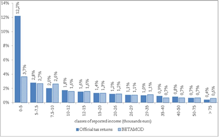

The 19% tax credits as a proportion of reported income (%).
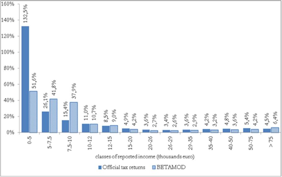

Social insurance contributions paid by self-employed individuals as a proportion of reported income (%).
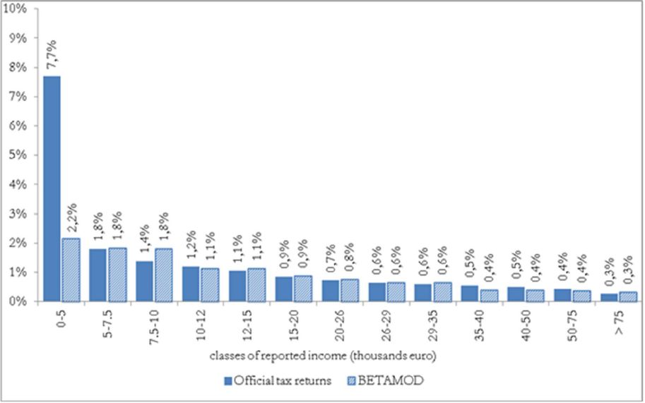
The 19% tax credit for healthcare expenses as a proportion of reported income (%).
References
-
1
Decomposing the Gini coefficient to reveal vertical, horizontal and reranking effects of income taxationNational Tax Journal 47:273–294.
-
2
Tax-Benefit Models, STICERD Occasional Paper, No. 10Grossing-up FES data for Tax-Benefit Models, Tax-Benefit Models, STICERD Occasional Paper, No. 10, London, London, School of Economics, STICERD.
-
3
The distributional effects of personal income tax expenditure, EUROMOD Working Paper Series, EM14/14University of Essex.
-
4
Estimating Nonnegative Matrices from Marginal DataInternational Economic Review 6:294–310.
-
5
Mapp, a tax benefit microsimulation Model for the Analysis of Public Policies in ItalyUniversity of Modena and Reggio Emilia, Department of Economics.
-
6
Household Income and Wealth in 2010, Supplements to the Statistical Bulletin, 6.Household Income and Wealth in 2010, Supplements to the Statistical Bulletin, 6..
-
7
Gli effetti redistributivi dell’evasione fiscale in ItaliaRicerche quantitative per la politica economica, Bank of Italy, Rome pp. 1–38.
-
8
The Siena microsimulation model (SM2) for net-gross conversion of Eu-Silc income variablesInternational Journal of Microsimulation 4:35–53.
-
9
Microsimulation as a tool for evaluating redistribution policiesJournal of Economic Inequality 4:77–106.
- 10
-
11
How Big Are Total Individual Income Tax Expenditures, and Who Benefits from Them?American Economic Review: Papers & Proceeding 98:79–83.
-
12
Mancate interviste e distorsione degli stimatori, Temi di discussione, 172, Banca d’Italia.Mancate interviste e distorsione degli stimatori, Temi di discussione, 172, Banca d’Italia..
-
13
The Importance of Choosing the Data Set for TaxBenefit AnalysisInternational Journal of Microsimulation 6:86–121.
-
14
Administrative and Survey Microdata on Self-Employment: the Italian Experience with the Eu-Silc project’, paper presented at the Iariw 29th General Conference, Joensuu, Finland, . pp. 20–26.
-
15
Integrazione dei dati campionari Eu-Silc con dati di fonte amministrativaCollana Istat Metodi e Norme, 39, Rome, March 2009.
-
16
The static microsimulation model of the Italian Department of Finance: Structure and first results regarding income and housing taxation, Economia Pubblica (forthcoming).The static microsimulation model of the Italian Department of Finance: Structure and first results regarding income and housing taxation, Economia Pubblica (forthcoming)..
-
17
The Construction of Gross Income Variables of EU-SILC (EU Statistics on Income and Living Conditions) in Italy: a mixed strategy using microsimulation and administrativePaper presented at the 2nd General Conference of the International Microsimulation Association: Microsimulation - Bridging data and Policy, June .
-
18
Grossing-up and validation issues in an Italian tax-benefit microsimulation model. Econpubblica WP, No. 117Milan: Bocconi University.
-
19
Tax Evasion in Italy: An Analysis Using a Tax-benefit Microsimulation ModelThe IUP Journal of Public Finance 4:19–37.
-
20
Health care is an individual necessity and a national luxury: applying multilevel decision models to the analysis of health care expendituresJournal of Health Economics 19:259–270.
-
21
Economia non osservata e flussi finanziari, Rapporto Finale, Ministero dell’Economia e delle Finanze, RomaEconomia non osservata e flussi finanziari, Rapporto Finale, Ministero dell’Economia e delle Finanze, Roma.
-
22
Imputation of gross amounts from net incomes in household surveys: An application using EUROMOD, EUROMOD Working Paper Series, EM1/01University of Essex.
- 23
-
24
Italy: The Delega Fiscale and the Strategic orientation of tax reformIMF Fiscal Affairs Department.
-
25
Tax Evasion and the Shadow EconomyPersonal Income Tax Evasion in Italy: An Estimate by Taxpayer Type, Tax Evasion and the Shadow Economy, Cheltenham, UK, Edward Elgar Publishing.
-
26
The impact of mortgage interest tax relief in the Netherlands, Sweden, Finland, Italy and Greece, EUROMOD Working Paper Series, EM2/07University of Essex.
-
27
Gruppo di lavoro sull’erosione fiscale: Relazione Finale, Roma, November 2011.Gruppo di lavoro sull’erosione fiscale: Relazione Finale, Roma, November 2011..
-
28
Microsimulation Modelling for Policy Analysis. Challenges and InnovationsCambridge: Cambridge University Press.
-
29
Medical care expenditure: A cross-national surveyJournal of Human Resources 12:115–125.
-
30
Developing a static microsimulation model for the analysis of housing taxation in ItalyInternational Journal of Microsimulation 4:73–85.
-
31
Redistributive effect of income taxation: Decomposing tax base and tax rates effectsBulletin of Economic Research 42:121–129.
- 32
-
33
The Central Role of the Propensity Score in Observational Studies for Causal EffectsBiometrika 70:41–55.
- 34
-
35
EUROMOD: the European Union tax-benefit microsimulation modelInternational Journal of Microsimulation 6:4–26.
-
36
Misure globali della progressività, dell’incidenza e della redistribuzione dell’imposta’, Statistiche Fiscali, Ministero dell’Economia e delle Finanze, Roma.Misure globali della progressività, dell’incidenza e della redistribuzione dell’imposta’, Statistiche Fiscali, Ministero dell’Economia e delle Finanze, Roma..
-
37
Reforming Tax Expenditures in Italy: What, Why, and How? IMF Staff Working paper, WP/14/7Reforming Tax Expenditures in Italy: What, Why, and How? IMF Staff Working paper, WP/14/7.
-
38
Redistribution, horizontal inequity and reranking: how to measure them properlyPublic Finance Review 36:563–587.
-
39
The redistributive effect and progressivity of taxes revisited: An International Comparison across the European Union, GINI Discussion Papers 88Amsterdam Institute for Advanced Labour Studies.
Article and author information
Author details
Acknowledgements
We thank Cesare Dosi, Devis Geron, Luciano Greco, Simone Pellegrino, Vincenzo Rebba, Tiziano Vecchiato, Michele Zanette, the editor and two anonymous referees for their useful comments. We are indebted to Fabrizia Lapecorella and Paolo Acciari (Ministry of Economy and Finance) for providing official tax returns data. Financial support from the Department of Economics at the Ca’ Foscari University of Venice is gratefully acknowledged. Data from the Survey of Income and Living Conditions, obtained through the Italian Office for National Statistics, have been used with permission.
Publication history
- Version of Record published: December 31, 2015 (version 1)
Copyright
© 2015, Vidyattama et al.
This article is distributed under the terms of the Creative Commons Attribution License, which permits unrestricted use and redistribution provided that the original author and source are credited.