A geospatial dynamic microsimulation model for household population projections
- Research Triangle Institute, United States
- Article
- Figures and data
-
Jump to
- Abstract
- 1. Introduction
- 2. FPOP: Components and processes
- 2.1 FPOP application to a U.S. population
- 2.2 Individual life events
- 2.3 Life events: household events
- 3. Computational infrastructure
- 4. The modeling framework and external model integration
- 5. Results-examples
- 6. Discussion
- Footnotes
- References
- Article and author information
Abstract
Forecasting Populations (FPOP) is a microsimulation model (MSM) that is the demographic core of an extensible modeling framework. The framework, with FPOP at its core, enables the geospatial projection of a population under purely demographic processes or under the additional influence of exogenous factors such as disease, policy changes and prevention programs, or environmental stressors. Empirically-derived transition probabilities of life events such as birth, death, marriage, divorce and migration, captured in lookup table format, drive the simulation. These transition probabilities can be modified dynamically by external user-defined functions or other external MSMs. The use of MSM structures and methodologies enables FPOP to portray the impact of heterogeneity in the geospatial dimension (e.g., distribution of environmental factors or distribution of intervention programs), as well as the social dimension (e.g., household or social network correlates), on the projections. POP is designed and structured to: enable linking with external MSMs of any kind; support inclusion or configuration of more detailed transition probabilities; be scalable to millions of agents; use either an existing baseline synthetic population or a custom synthetic population of the user’s design; and, run under computing environments that don’t require a high degree of specialized software or hardware. In this paper we describe the design and structure of FPOP and then apply FPOP first under purely demographic processes and, secondly, in conjunction with an external disease model of obesity.
The objective of FPOP is to provide a demographically realistic projection of the size, structure, and movement of populations and households decades into the future.
1. Introduction
Understanding and predicting trends in population composition, structure, and location are of interest to researchers, decision makers, and scientists in government and industry (NAS 1991; Geard 2013). MSMs were first introduced fifty years ago by Orcutt to refine existing models regarding the predicted effects of various governmental socioeconomic policies on the “behavior of elemental decision-making units” such as individuals, households, and firms (Orcutt 1957:136). These techniques model the dynamics of a population by simulating change in the demographic and social behaviors of its micro-units over the life course. MSMs provide a powerful analytic tool for exploring how populations may behave in the future as they can capture the heterogeneity inherent in a population due to social factors (such as household or familial attributes) that either affect or are affected by the risk from external phenomena of interest (NAS 1991, 2011).
Dynamic MSMs, which incorporate changes in behaviors that impact life event probabilities, historically have been developed to better understand the effects of various social and economic policies on individuals and households. Models such as PENSIM (Holmer et al., 2014), APPSIM (Harding 2007), SESIM (Klevmarken 2010), DESTINIE 2 (Blanchet 2009) and MIDAS (Dekkers et al., 2012) have been used to evaluate future consequences of demographic aging, potential changes in national pension policies and/or their consequences for intergenerational wealth redistribution. More recently, models have been extended to explore health outcomes (Luke and Stamatakis, 2013), such as infectious disease transmission and spread (Eubank 2004; Ferguson et al., 2006; Longini 2007; Cooley 2008; Lee 2010; Geard 2013), obesity (van Baal et al., 2008; Lymer 2012], the effects of tobacco control policies on smoking (Goldstone 2005), and in the evaluation of screening recommendations on breast and prostate cancer (CISNET Cancer Intervention and Surveillance Modeling Network, CISNET.gov) (see review by Rutter 2011; Kopec 2012). However, few examples exist of general purpose dynamic MSMs that incorporate geospatial, household structure, and individual level attributes for projecting patterns of population change over long periods of time. For social processes that occur over long time frames, MSMs offer the flexibility to investigate, for example, inter-relationships among individuals (e.g., sexual behaviors and treatment compliance), causal factors (treatment effectiveness), and disease traits (secondary infection rates and genetic mutation rates) over time (Zaidi 2009; Zucchelli 2010).
In this paper, we describe a dynamic MSM called FPOP that was developed as the demographic core to a modeling framework that projects the geospatial distribution of microdata populations into the future and allows linkage to various externally-defined and independently functioning modules, ex., health or environmental events, disease, economic factors. Using an iterative process, these modules influence population size, structure, and characteristics independently of FPOP’s empirically-derived demographic core components. When linked to an exogenous MSM (such as a chronic disease model) we illustrate how the health status of the individuals derived from the disease model updates life event probabilities for FPOP. Prevention strategies can be layered as an additional component onto the disease model to evaluate the combined impact on future populations. The overarching goal of FPOP is to capture the effects of demographic change on the household and population structure over arbitrarily long periods into the future. Because the transition probabilities are defined externally and the framework architecture is modular, FPOP does not need to be modified to run in alternative frameworks representing other populations or non-health scenarios.
2. FPOP: Components and processes
FPOP is a dynamic, discrete-time MSM that incorporates linkages between life events, changes in household structure and changes in the attributes of individuals and their location as part of the aging process. Individuals can be tracked over the life course for decades. The life events that modify households and populations include aging, mortality, birth, marriage/union formation and dissolution, and migration. The occurrence of life events for each individual at each discrete time step is determined stochastically by transition probabilities that subsequently can be modified during the course of the simulation. Life events occur by generating a random value from a uniform probability distribution with range [0,1] and comparing that value with the individual’s event-specific probability. If the random value is smaller or equal to the probability then the event occurs; otherwise, there is no change in status. Transition probabilities may be specified as tables or functions and are presented to FPOP as external files.
Our design allows users to specify the duration and time step of any FPOP simulation in any combination of days, weeks, months, and years. FPOP is structured so that at each time step, the six different demographic processes are randomly determined for each individual, household by household. Individuals may be removed from the model based on estimated mortality or emigration rates, and added to the population based on estimated fertility and immigration rates. The data modified by the individual transitions at the end of time t are passed to the intermediate (in our case, disease) model, if it is included. If no intermediate model is included, the FPOP data at the end of time t form the input data for the next time period, t + 1, and so forth.
Transition probabilities for all demographic events are automatically scaled at runtime based on the ratio between the time step size and the temporal resolution of the probabilities (metadata about the native temporal scale of the probabilities are required inputs to FPOP). The model assumes that each demographic event may only occur once per time step, thus limiting the time step size to less than or equal to the smallest temporal resolution of all the demographic events. This allows input probabilities to remain within the appropriate range [0, 1] and eliminates the need to handle potentially complex outcomes (at both the individual and household level) arising from multiple occurrences of the same event in the same time step.
FPOP’s life event probabilities are input as ASCII, comma-separated text files that can be easily modified to test alternate policy and demographic scenarios using externally defined functions. These FPOP probability lookup tables contain select synthetic person attributes and metadata that specify which synthetic attributes should be accessed at runtime to perform the probability lookups. Because these text files drive the generic routines within FPOP for matching a synthetic individual with a demographic event probability, researchers are able to configure multidimensional probability lookup tables according to the availability of data. It is also through these life event probabilities that external models can impact the population projection. For instance, external model estimates of the effectiveness of various interventions may modify individual probabilities of death and therefore the overall future size, composition, and distribution of the population. External model effects can be readily accommodated, independent of FPOP’s dynamic population aging structure.
2.1 FPOP application to a U.S. population
To illustrate FPOP, we initially link the model to an existing, spatially-explicit synthetic baseline population—including individuals, households, and locations—that is representative of the U.S. household population in 2010. These microdata can be downloaded for free by state or county, allowing researchers to model any study area in the U.S. or the entire U.S. population (Wheaton 2014). Initial transition probabilities are statistically calculated using Census, Vital Statistics, or survey data or tabulated directly from published sources. Table 1 lists each of the demographic parameters included in the U.S. version of FPOP, the data used to initialize each transition probability, and the individual characteristics used to define each probability. The selection of explanatory variables is driven by the availability of data and the association of the variables with the outcome of interest. If a functional form version of transition probabilities is used, regressions may include other relevant explanatory variables. At a minimum, transition probabilities are estimated according to individual characteristics that include age, sex, race and Hispanic origin (classified as Non-Hispanic white, Non-Hispanic black, Hispanic, and other), and geographic location. These key variables are generally available for tabulation from all of the data sources.
Initial demographic parameters applied to FPOP for a U.S. population.
| Parameter | Source of estimate | Geospatial level of estimate | Statistical model | Explanatory variables |
|---|---|---|---|---|
| Aging | 2007–2011 ACS | Time t -> t+1 | ||
| Mortality | NCHS/NVSS | National | Lifetable | Age, sex, race, Hispanic origin |
| Fertility | NCHS/NVSS | State | Age-race-parity specific probability | Age, race, parity Hispanic origin |
| Union | ||||
| Formation | ACS 2009 | State | Logistic regression | Age, sex, race Hispanic origin, education, employment, |
| Dissolution | ACS 2009 | State | Logistic regression | Age, sex, race, Hispanic origin, education, employment |
| Migration | ACS 2009; 2008–10 | State | Logistic regression | Age, sex, race, Hispanic origin |
-
ACS is the American Community Survey; NCHS NVSS is the National Center for Health Statistics / National Vital Statistics System.
For most processes, probabilities are generated at the State level. The consequence is that several life events are interdependent with location. For example, the likelihood that a Hispanic 20-year old woman living in California will give birth is x. Whereas, if she lives in a different State, the probability of her giving birth is y1.
For the U.S. simulation, each household consists of a primary householder or household head (at least 15 years of age), alone or in combination with other family or non-family members. Family households include at least one additional individual who is related to the household head by birth or marriage (adoption is disregarded in the model). Family households are defined as married/cohabiting couple, married/cohabiting couple with family, and single householder with family. Nonfamily households may include only one person – a single-person household -- or unrelated adults sharing a household (e.g. roommates)2. Each demographic event – fertility, mortality, union formation and dissolution, migration – may potentially affect the size and composition of the household.
2.2 Individual life events
Mortality probabilities are assessed by single year of age up to a maximum age of 100 years. Race, age- and sex-specific mortality rates are presented for Hispanic, Black, and White, with “Other” race/ethnic groups set equal to probabilities for all races combined. The source probability data are annualized (i.e., the probability estimates the likelihood of an event occurring in one year (NCHS 2012)). But FPOP will adjust annual probabilities automatically for time steps with duration less than the time step implicit in the data by scaling down the given annual probability values.
In addition to removing individuals from the simulation model, deaths trigger both personal and household changes. For instance, when death occurs to a spouse, the marital status of the surviving spouse is changed to ‘widow’ and a new household head is assigned (if appropriate). If death occurs to a single-person residing alone, the household is removed from the model.
Fertility estimates are calculated from 2008 birth data (NCHS 2013) and Census state-level data (U.S. Census 2013). We predict the conditional probability of giving birth in a particular year based on a woman’s parity3. Using birth counts by single year of age from the NVSS and intercensal population estimates for women aged 15 to 44 years from the U.S. Census, overall birth rates are tabulated and then adjusted based on the parity distribution of women in 2008 by exact age 15 to 44 years for three race groups -- white, black, and all races -- and Hispanics. Our model assumes a maximum number of five births and a minimum interval of 9 months between childbirth in the same woman.
Once a woman in the synthetic population has been selected to give birth, whether she has a single birth or multiple births is determined based on multiple birth rates observed in the U.S. for the period 2005–08 (NCHS 2009). The sex of the child(ren) is assigned using a separate random process. The U.S. sex ratio at birth, 105:100, is used to determine the sex of the child. The race of child is assigned based on mother’s race, which is consistent with the national statistics.
When FPOP determines that a birth occurs, the child or children born are assigned to the mother’s household. The household size is increased by the number of children born. First births result in reclassification of household to single-person with children, married couple with children or cohabiting couple with children. The newborn child or children are assigned a date of birth. For the selected year of birth, FPOP chooses a birth date at random based on the time step interval. If the time step is one year, then one of 365 possible days will be assigned as the birth day.
2.3 Life events: household events
This version of FPOP focuses on two key union events: probability of marriage in the past simulated time interval (among those aged 15+) and probability of divorce in the past time interval (among those ever married and aged 15+). We calculate estimates of marriage and divorce in the past year by race/ethnicity, sex, age, and State using logistic regression models with additional controls for education and current employment. Cohabitation status as well as same-sex marriages will be considered in the next version of FPOP; as a consequence our union estimates likely underestimate union formation and dissolution.
Developing a dynamic microsimulation that considers the formation of partnerships involves an additional issue: whether or not the partner is identified within the model population, i.e., an ‘open’ model versus a ‘closed’ model (see Morand et al., 2010). Partnership selection in FPOP is ‘closed’, i.e., partners for individuals ‘tagged’ for marriage/union based on our initial probabilities are found among existing eligible population members. Couples are matched based on their age, race, and education using tabulations of couple characteristics at the national level from the 2006–10 National Survey of Family Growth (tabulations prepared by NCHS staff, April 2013). Male and female partner characteristics among currently married and/or currently cohabiting couples aged 15 to 44 years based on age (same, 1 to 3 years difference, 4 to 6 years difference, 7 or more years difference), race and Hispanic origin, and education (more, less, or same) were used to identify eligible partners. Rather than a dual-mate matching process, where the optimal partner is selected to satisfy both partners, we apply a simpler unidirectional selection process of finding a mate that satisfies the criteria for the tagged individual. The approach is heuristic – the first suitable mate based on our matching criteria is selected. Not all tagged individuals are assigned a mate; if no suitable match appears, he or she may re-enter the potential marriage pool at the next time step based on his or her recalculated marriage/union probability (see Walker and Davis, 2013).
When FPOP determines that a person is to form a new union, a number of changes at the household-level occur. For couples who marry, new households may be formed or existing households expanded if one of the members of the couple already has children.
Likewise, when FPOP determines that a person who is in a union or marriage should dissolve that partnership, both partners are classified as “divorced.” Upon dissolution, households are reallocated based on couples’ characteristics. For couples with children who divorce, children within the household are randomly assigned to one of the parents with the assumption that 90 percent will stay with the mother.
2.4 Geographic events and location (Internal migration, Immigration, and Emigration)
We tabulate the probability of moving within the past year for the population aged one year and older by age, race/Hispanic origin, sex, and State of residence. State-to-State migration in-flows and out-flows (internal migration) are tabulated and include the number of non-movers (same residence one year ago), the number of movers within the State, and the number of movers to each of the other States. Emigration is defined as the number of people who move outside the country. These migration estimates are calculated in two stages. In the first stage, the probability of moving within the last year for the population aged one year or more is estimated. In the second stage, for those who moved, where they moved (same State, different State, out of country) is determined. Currently, simulation of migration for the examples we provide is limited to person level movements within and between States. However, this is strictly a limitation of available data. FPOP can simulate the migration of households or persons within and between any unit of geography such as county if those data are used.
For immigration from outside the country, a simpler procedure is implemented that assumes a 1% annual net immigration rate, although the FPOP structure can accommodate any user-defined value.
When a synthetic agent migrates to a region that is outside of an FPOP run’s spatial domain, they are removed from the population entirely and cannot return.
Internal migration within a given simulation geographic study area results in an existing synthetic person being assigned a new location. Immigration from outside a given simulation study area occurs in FPOP through a simple copying mechanism. In this case, a static rate determines what percent of the current total population should be copied at each time step. Synthetic agents are chosen using uniform random selection until the required number of new synthetic agents has been selected. The characteristics of the copied agents do not change. If suitable data on the characteristics of migrants was available, then assignment of custom individual attributes could be readily incorporated into FPOP. No new households are created during this process.
The 2010 Synthetic Population used to initialize FPOP includes a location of each synthetic household based on EPA’s ICLUS 90-meter population estimates (EPA, 2009). As the population ages in the FPOP simulation, newly created households need to be provided with realistic locations. Currently, FPOP determines the State and county for each new household, but does not derive an individual latitude/longitude coordinate for it4.
3. Computational infrastructure
Software environment: FPOP is written in the open-source Python programming language.
Generic, open source data storage: FPOP stores synthetic population records in a MongoDB (https://www.mongodb.org) database. Unlike in a relational database, MongoDB data records (known as “documents”) need not conform to a schema. This greatly simplifies the storage of synthetic population variables and allows populations (and sub-populations) with dissimilar attributes to be stored in MongoDB and accessed with generic routines.
Dynamic life event probabilities: Event-specific probabilities are stored in ASCII, comma-separated text files that can be modified easily. These FPOP probability lookup tables contain select synthetic person attributes and metadata that specifies which synthetic attributes should be accessed at runtime to perform the probability lookups. Because these text files drive the generic routines within FPOP for matching a synthetic individual with a demographic event probability, researchers are able to configure multi-dimensional probability lookup tables according to the availability of data.
FPOP also provides the ability to adjust probability lookups dynamically during a simulation using externally defined functions or tables. With these functions it is possible to modify any probability based on (1) select attributes of the individual, (2) the current time step number and (3) basic conditional logic (such as “if- then-else” constructs). This feature allows FPOP to adjust probabilities for all individuals in the population or for highly selective sub-populations, at all times or specific simulation periods.
Simulation runtime scalability: A key challenge to projecting synthetic populations is the range and potential magnitude of their sizes. FPOP employs a scalable, parallel design implemented in the Python programming language that allows it to simulate the smallest or the largest of these geographies with efficiency proportional to the size of the population and amount of compute nodes allocated to each simulation run. Central to this design is a “map-reduce” strategy with the following components:
FPOP “maps” the synthetic population by evenly distributing synthetic households across multiple compute nodes. At each time step, all nodes check their sub-populations in parallel to one another for demographic events. Workload is balanced across all nodes by distributing the population using uniform random selection, to assure that each node is able to complete an entire set of simulated life events in roughly the same amount of time as all other nodes.
FPOP “reduces” the results of each time step by sending the results of each node to a single, dedicated processor which serves as the FPOP controller. The FPOP controller aggregates results for each sub-population into population-wide results (such as population size, number of births, deaths, etc.).
Note that all FPOP processes communicate over standard network protocols and must also be able to connect to the networked MongoDB server.
Because FPOP does not utilize a formal MapReduce framework such as Hadoop, (https://en.wikipedia.org/wiki/MapReduce) it does not require a specialized distributed file system like Hadoop’s HDFS. We find it useful that FPOP can run on any networked hardware where the Python programming language is supported without an additional external framework. FPOP exists as a parallelized process. Overall speed of the model depends on the size of the population, the number of nodes running the process, the timestep selected and the number of timesteps simulated. Historically, we have limited the populations per node to slightly more than 300,000 persons per node. Our estimates indicate that FPOP processes a population of this size in slightly less than 27 seconds per time step. Thus, a population of 9 million that is projected in annual time steps 30 years into the future and operates on 30 nodes would complete processing in 27*30 operations in 810 seconds or around 13 minutes.
4. The modeling framework and external model integration
For the implementation described here, we use FPOP with the baseline synthetic U.S. population coupled with individual probabilities of key life events (births, deaths, union formation/dissolution, migration, and aging) to forecast populations. The FPOP MSM framework, however, enables linkages to additional populations and to additional external models that dynamically interact on an iterative basis (Figure 1). As an example of this extensible framework, we link FPOP to an external model of a chronic disease, obesity, to investigate the effectiveness of a prevention program based on body mass index (BMI). We apply this extended model to a population of Indonesian adults. A model of obesity was chosen because the effects of obesity on health often occur over long time periods. In total, the models address demographic changes (FPOP), disease state (obesity, BMI), and mitigation and intervention strategies (prevention program). In each iteration, the models pass the population with its associated social structure (household and distance to health care settings where intervention programs are provided), personal attributes, and geospatial information, updating the population and modifying parameters for the other models, as appropriate.
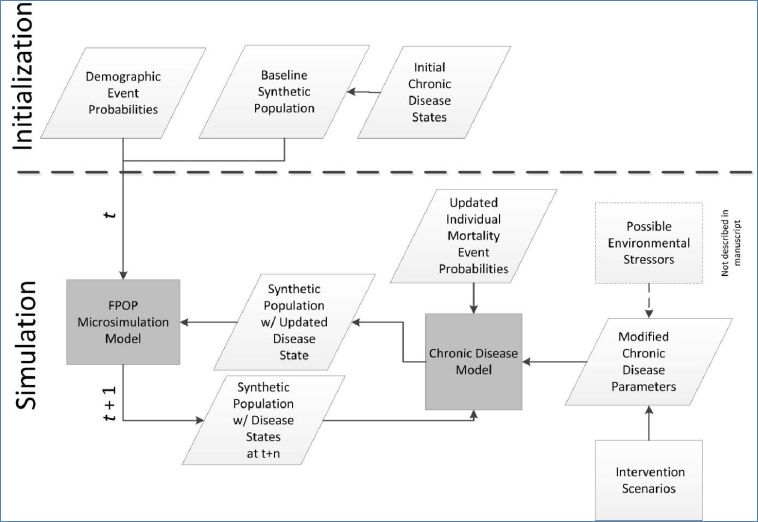
A model framework showing FPOP as the demographic core for a chronic disease scenario.
The rationale behind implementing an obesity model is that BMI is an indicator of nutritional status and that changes to BMI over time reflect changes in overall levels of obesity. Thus, predictions of future numbers of people with high levels of BMI can be used to indicate to both policy makers and the community at large the potential scale of the obesity epidemic and whether proposed interventions are effective in containing the epidemic. The obesity model also dynamically effects the FPOP model because increases in obese populations modify the mortality probabilities in FPOP, hence changing the underlying synthetic population over time.
In the next section, we present results demonstrating: 1) FPOP as the demographic core of our modelling framework in one U.S. State, North Carolina, and 2) the interaction of the FPOP core framework with external models of obesity and a hypothetical intervention program to reduce individual BMI levels among adults residing in one province of Indonesia, Yogyakarta.
5. Results-examples
5.1 FPOP demographic core: North Carolina
We present model results for the State of North Carolina running FPOP solely with demographic projection processes. We simulate a synthetic population of 9.5 million persons in 2011 and apply each of our event-specific probabilities at annual time steps through 2050. Figure 2 illustrates FPOP output of the simulated age structure (using four broad age groupings) for the period 2011–2050. Although any age groupings can be chosen, these categories are typically used to illustrate dependency ratios or the ratio of the combined child and aged population to the population of intermediate age. Of note is the increasing proportion of elderly persons, largely consistent with population effects of the aging baby boom generation. By 2030, an estimated 20% of North Carolinians will be aged 65+ compared to 13% in 2011.
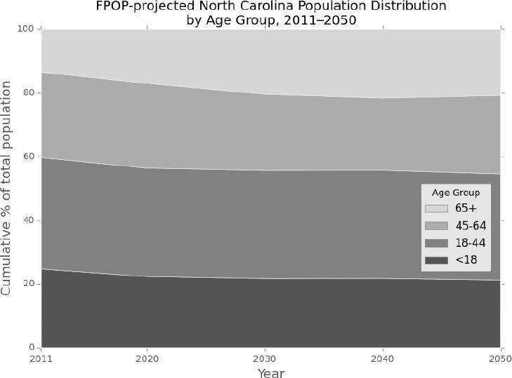
Projected age distribution of North Carolina, 2011–2050: FPOP.
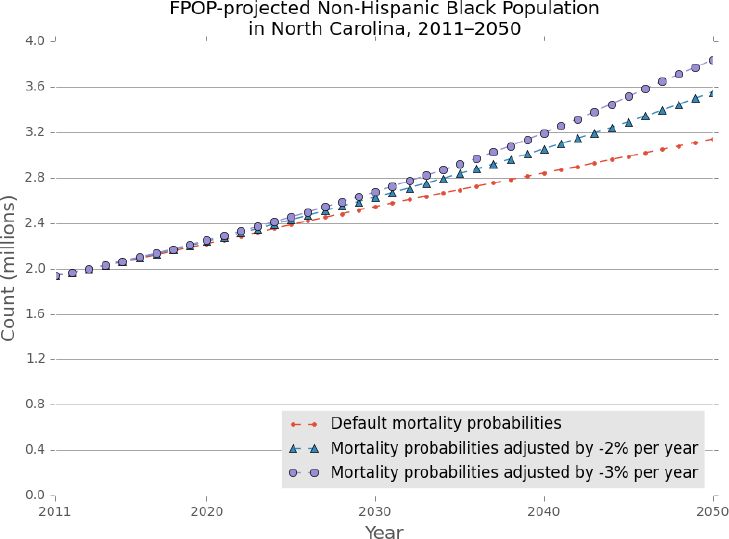
Next we illustrate FPOP’s flexibility to incorporate various externally-defined functions to test alternative demographic scenarios and transition probabilities. Figure 3 illustrates the effects on population growth of introducing a two percent and a three percent annual reduction in non-Hispanic Black mortality rates at baseline – all other key events remain unchanged. FPOP allows the user to modify event probabilities for population subgroups, while maintaining the original transition probabilities for the remaining population. In this instance, we assess the overall population effects of projected sustained improvement in Black mortality (among all age groups) across the entire projection period and note the overall projected increases in Black population relative to the default probabilities.

Projected non-Hispanic Black population, North Carolina 2011–2050 with default and adjusted mortality probabilities.
To assess whether the model could generate output consistent with official demographic projections, we compared FPOP results with those provided by the State of North Carolina. The State Demographics Branch of the North Carolina Office of State Budget and Management (NC OSBM) routinely publishes annual state and county population projections for local economic planning and resource distribution (NC OSBM 2013). Current estimates project through the year 2033 and were published in September 2013. We compare our synthetic output from FPOP with published data using time series trends from NC OSBM.
Figure 4 compares annual population totals projected by FPOP for North Carolina with those published by the NC OSBM. Total population counts in FPOP and the State were similar across the time period, differing by less than one percent in 2020 and less than three percent in 2030. The population was projected to increase 30.3% in FPOP compared to 25.3% in NC OSBM.
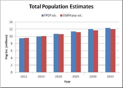
Population projections, North Carolina 2011–2033: FPOP and NC OSBM.
Trends in age structure were nearly identical (Figure 5). The population aged 65+ increases steadily across the projected time period; by 2033, an estimated one in five residents will be aged 65 years or older. Population estimates by age varied by less than 0.4% across all age groups.

Trends in age structure by age groups, North Carolina 2011–2033: FPOP and NC OSBM.
According to population estimates, during the last two decades population growth in North Carolina has been driven largely by net in-migration into the state, resulting in relatively large, growing and youthful urban centers (CPC 2013). This trend is expected to continue at least for the short term (Table 2). Population natural increase due to excessive births relative to deaths over the next two decades is expected to continue to slowly decline, with migration contributing to a larger share of population change. Compared to the NC OSBM, FPOP projects slightly higher fertility (although fertility rates in both projections remain low) and in-migration resulting in higher population counts.
Components of population growth, North Carolina 2011–2033: FPOP and NC OSBM.
| Base Pop (2011 FPOP, 2010OSBM | Nat. Incr. | Net in-migration | Projected 2020 Pop | Nat. Incr. | Net in-migration | Projected 2030 Pop | Nat. Incr. | Net inmigration | Projected 2033 Pop | |
|---|---|---|---|---|---|---|---|---|---|---|
| 2010(1)–2020 | 2020–2030 | 2030–2033 | ||||||||
| FPOP Projections, 2011–2033 | 9,490,337 | 336,507 3.55% | 863,210 9.10% | 10,690,054 | 187,820 1.76% | 1,128,992 10.56% | 12,006,866 | 2,058 0.02% | 363,861 3.03% | 12,372,785 |
| NC OSBM, 2010–2033 | 9,535,471 | 319,121 3.35% | 762,267 7.99% | 10,616,859 | 166,140 1.56% | 899,263 8.47% | 11,682,262 | 16,607 0.14% | 301,691 2.58% | 12,000,560 |
| Ratio: OSBM/FPOP Projections | 1.005 | 0.993 | 0.973 | 0.970 | ||||||
-
Nat. Incr.: Natural Increase=Births-Deaths; NC OSBM projections tabulated for 10-year periods beginning April 2010 and ending July 2033. FPOP estimates tabulated for 10-year periods beginning April 2011 and ending April 2033.
These results suggest that at least with regard to total population size and structure, our synthetic estimates coincide with projections prepared by the NC-OSBM for 2011–2033.
5.2 Indonesia obesity model
As a second illustration, we apply FPOP to a baseline synthetic population of Indonesia generated from a microdata sample of the Indonesian 2010 census which was replicated to create a 100% synthetic population. Each individual is described by a number of characteristics including but not limited to sex, age, race, ethnicity, education, and family type (Minnesota Population Center, http://www.ipums.org). Transition probabilities simulating fertility, mortality, and aging derived from Census and survey data are applied over user-defined time steps for each synthetic individual while tracking corresponding changes in household composition, location, and size.
We link to the FPOP demographic core model two additional models: an ‘obesity baseline’ model assigning nutritional state and BMI to each individual and an obesity prevention model structured on improvements to diet. Each nutritional state – poor, neutral, and healthy -- has an associated mortality probability, and persons aged 25 years and over are assigned to a state according to their BMI status. Baseline BMI estimates are calculated for each individual based on age, sex, and urban/rural status using data from the Indonesian Family Life Survey (IFLS) a large ongoing longitudinal survey in Indonesia (Rand, 2014). The obesity prevention model was structured on diet programs designed to limit intake of total fats, free sugars, and sodium and increase consumption of fruits and vegetables, legumes, whole grains, and nuts. We translated this into a hypothetical behavioral intervention that consisted of a period of reduced caloric intake followed by a maintenance period. Specifically, this resulted in a modest mean 3-kg weight loss distributed over a 1-year period plus a 1-year maintenance period. After the intervention, individuals resumed their previous annual weight trajectory.
We ran FPOP with the linked obesity and intervention models for one Indonesian province, Yogyakarta, 50 years into the future. The purpose of this investigation was to assess the impact of specific changes in nutritional states on future obesity trends and the resultant morbidity and mortality profiles. We simulate changes to BMI over time. When an individual’s BMI levels reach specified levels, subjects move into a new nutritional state. We assume that post-intervention, a subject will remain in the healthy nutritional state for a fixed period of 1 year. As time advances subjects move from healthy to neutral or poor according to the change in their BMI.
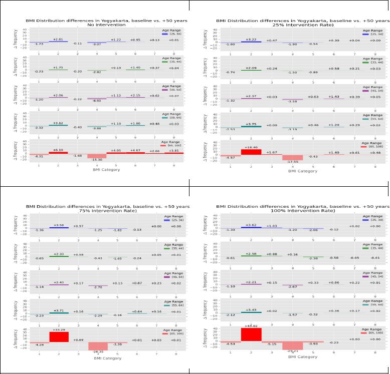
Participation in the intervention resulted in substantial decreases in the high end of the BMI distribution for all age groups, indicating substantial reductions in predicted BMI. Figure 6 displays the estimated change between baseline and 50 years in the future for each octile of BMI in Yogyakarta (octiles are defined as equal intervals on the scale bounded by a defined maximum and minimum). Each panel corresponds to a rate of intervention participation from 0%, 25%, 75%, and 100%.

Estimated change in body mass index (BMI) for men and women in urban and rural settings by different participation rates in intervention programs.
Increasing intervention participation rates increase the proportion of the population in the BMI octile 2, which is a favorable BMI, across all age groups. Without intervention, there is some increase in the obese (higher octiles) segment of the population. However, with intervention, there is a noticeable decrease in, for instance, BMI octile 4. Among those aged 45–54 years in BMI octile 4, for example, the BMI distribution difference between baseline and 50 years with no intervention is −4.6 points, whereas with 25% intervention participation, the point difference declines to −3.58 and with 100% participation, to an estimated difference of −2.67.
In sum, the Indonesia study illustrated the effectiveness of linking FPOP to a chronic disease model and interventions to create a simulation in which the chronic disease, potential interventions, and life events interact to provide a realistic simulation of this complex system.
6. Discussion
Population projection models allow investigators to simulate future population structure and change providing a useful tool for the evaluation of population effects of various health and social programs. FPOP incorporates geospatial, household structure, and individual-level attributes to provide realistic projections of the future size, composition, and movement of populations. FPOP was designed to be relatively simple, with reasonable data and computational requirements and the ability to link to external models of broad interest. In addition, FPOP is highly scalable. Changes in life events, determined by empirically-derived transition probabilities and captured in lookup table format, can be modified dynamically in FPOP by either externally-defined functions or other modules in the modeling environment. Users who have more geospatially specific, more recent, or more detailed transition probability data can easily incorporate that data into their FPOP runs. As part of the external models linkage process, FPOP can both affect and be affected by processes that occur within the external models.
Numerous MSMs and multi-state models have been developed over the past several decades spurred in large part by enhanced modeling techniques and the quality of available data to parameterize those models (for a review see Li, 2013). FPOP offers a flexible tool because both the baseline population and the transition probabilities are external. A FPOP implementation may use any synthetic microdata database or administrative or census data of actual individuals that contains both household and person-level characteristics as its baseline and the associated description of transition probabilities for significant life events. For illustration, we first selected a synthetic population for North Carolina from the publicly available U.S. 2010 Synthetic Population5 with FPOP transition probabilities defined from survey and vital statistics data. The North Carolina baseline population includes 9.5 million individuals and 3.74 million households—each with a specific set of latitude/longitude coordinates. We subsequently extended the FPOP model to project the population effects of an obesity prevention program on adults in Yogyakarta, Indonesia using a baseline population representative of every household and household occupant and their location. The external models linkage feature of FPOP allows geospatial and temporal projection of populations in response to various externally-defined and independently functioning modules, ex., health or environmental events, disease, economic factors. Although MSMs that simulate both spatial and household characteristics exist, for instance, SMILE (O’Donoghue 2011), SimBritain (Ballas 2005), SVIERGE (Holm 2008), these models simulate specific populations (i.e., household residents of Ireland, Britain, and Sweden) and were developed to address specific policy questions.
FPOP also contrasts with macrosimulation models and traditional demographic methods, such as the cohort-component method for population projections. The cohort-component method treats each cohort as a homogenous group, as opposed to individuals independently, and uses average probabilities of fertility, mortality, and migration, as opposed to individual probabilities based on personal characteristics which stochastically drive the determination of a demographic event. With consideration of multiple individual attributes, ex., age, sex, race, and ethnicity, etc., the computational requirements using the cohort-component method become complex since each combination of attributes must be tracked (Van Imhoff 1998). FPOP performs well even with large numbers of attributes, both individual and household, and can be based on an entire population, not a sample. Multi-state demographic projection methods have been developed but to our knowledge they do not offer the flexibility of FPOP or the ability to link to external models.
The functionality of FPOP and the built-in interactive capabilities to pass both the population and access new transition probabilities means that it can be linked in a modeling framework to a wide range of external models. The purpose of the external models is to represent changes to the life events that result from “interventions” that are introduced into the simulated population and that are not reflected in the baseline transition probability data, such as a new treatment for a chronic disease. Linkage to external disease models allow users, for example, to investigate heterogeneity in individual characteristics influencing disease onset and persistence over time, to quantify and forecast future independent effects of potential disease interventions on mortality, and to examine how change from one demographic state to another impacts disease outcomes over an individual’s lifetime. The flexibility of our approach and its research value arises from the design of the system, which allows those external models to influence population size, structure, and characteristics independently of FPOP’s empirically-derived demographic core components. This coupled system provides significant advantages over models that employ static aging and models that include limited interaction between demographic, behavioral, and disease characteristics.
Whereas MSMs provide useful methods for projecting population patterns over time, there are limitations. FPOP is dependent on parameters that are calculated from existing data. The quality of those data is intricately related to the validity of the model. Furthermore, these key life event probabilities are rarely static over long periods and the current model currently includes only a select number of events. Future model enhancements to FPOP include additional individual and household-level attributes and model parameters. Access to vital statistics microdata beginning with the year 2005 which includes a greater level of geographic detail has been acquired, permitting further refinements in terms of geography and time to measures of fertility and mortality. We will also incorporate measures of cohabitation and same-sex unions, important demographic trends that are likely to influence future population trends in the U.S. and other countries.
Footnotes
1.
Future versions of FPOP will incorporate more spatially refined (e.g., county-level) estimates generated from non-public use Census and Vital Statistics data. Additional parameters to be incorporated in future versions of FPOP include leaving the parental home, labor force status, cohabitation, and same-sex unions.
2.
This version of FPOP does not distinguish between married and cohabiting couples.
3.
Union status and duration and parity are important determinants of future fertility and often inter-correlated; we chose parity, the number of children previously born alive to a woman, as an explanatory variable in this version of the model.
4.
Enhancements to FPOP will include the use of ICLUS future population distributions to guide the placement of new households generated in FPOP.
5.
References
-
1
SimBritain: A spatial microsimulation approach to population dynamicsPopulation, Space and Place 11 pp. 13–34.
-
2
Creating Synthetic Baseline PopulationsTransportation Research Part A: Policy and Practice 30:415–429.
-
3
The Destinie 2 microsimulation model: increased flexibility and adaptation to users’ needsConference of the International Microsimulation Assocation 2009.
- 4
-
5
Population growth and population aging in North Carolina countiesAccessed February 12, 2014.
-
6
Using Influenza-Like Illness Data to Reconstruct an Influenza OutbreakMathematical and Computer Modeling 48:929–939.
-
7
Alignment and matching in multi-purpose household modelsIntl Jour of Microsimulation 3:34–45.
-
8
Dynamic microsimulation modeling for policy support: An application to Belgium and possibilities for JapanRev Socionetwork Strat 6:31–47.
-
9
Guidance on the Development, Evaluation, and Application of Environmental Models EPA/100/K-09/003Guidance on the Development, Evaluation, and Application of Environmental Models EPA/100/K-09/003.
- 10
-
11
A primer on the Dynamic Microsimulation Income Model (DYNASIM3)Washington, DC: Urban Institute.
- 12
-
13
Synthetic Population Dynamics: A model of household demographyJournal of Artificial Societies and Simulation 16:8.
-
14
Discrete-time and continuous-time approaches to dynamic microsimulation reconsidered. Technical paper 13Canberra, Australia: National Center for Social and Economic Modeling.
- 15
-
16
APPSIM: The Australian Dynamic Population and Policy Microsimulation ModelAustralia: National Centre for Social and Economic Modeling, Canberra.
-
17
The SVERIGE Spatial Microsimulation Model, Discussion paper 595Umea University: Department of Social and Economic Geography.
- 18
-
19
Australians over the next 50 years: providing useful projectionsAustralia: National Centre for Social and Economic Modeling, Canberra.
-
20
Microsimulation for public policy: Experiences from the Swedish model SESIM. Economic and Social Research Discussion Paper Series No. 242Microsimulation for public policy: Experiences from the Swedish model SESIM. Economic and Social Research Discussion Paper Series No. 242, Tokyo, Japan.
-
21
Advances in microsimulation modeling of population health determinants, diseases, and outcomes, Epidemiologic Research International1–3, et al.
-
22
Staphylococcus aureus vaccine for orthopedic patients: An economic model and analysisVaccine 28:2465–2471.
-
23
Simulation models of obesity: A review of the literature and implications for research and policyObesity Reviews 12:378–94.https://doi.org/10.1111/j.1467-789X.2010.00804.x
-
24
A survey of dynamic microsimulation models: uses, model structure, methodologyInternational Journal of Microsimulation 6:3–55.
-
25
Containing a large bioterrorist smallpox attack: A computer simulation approachInternational Journal of Infectious Diseases 11:98–1.
-
26
Systems Science Methods in Public Health: Dynamics, Networks, and AgentsAnnual Review of Public Health 33:357–376.
-
27
Developing a dynamic microsimulation model of the Australian population: a means to explore obesity impacts over the next 50 yearsEpidemiology Research international.
-
28
Trend Analysis of the Sex Ratio at Birth in the United StatesNational Vital Statistics Reports, 53, 20.
-
29
Demographic modeling: the state of the artParis: Institut National Etudes Démographiques (INED).
-
30
For the Public’s Health: The Role of Measurement in Action and AccountabilityWashington DC: National Academy Press.
-
31
Understanding the Changing Planet: Strategic Directions for the Geographic SciencesWashington DC: National Academy Press.
- 32
- 33
- 34
- 35
- 36
- 37
-
38
Division of Vital Statistics, National Center for Health StatisticsAccessed January 17, 2013.
-
39
Dynamic Microsimulation – A Methodological SurveyBrazilian Electronic Journal of Economics.
- 40
- 41
- 42
-
43
Dynamic microsimulation models for health: A reviewMed Decis Making 31:109–18.https://doi.org/10.1177/0272989X10369005
- 44
- 45
-
46
Lifetime medical costs of obesity: prevention no cure for increasing health expenditurePlos Med 5:e29.
- 47
-
48
Microsimulation of Urban Development and Location Choices: Design and Implementation of UrbanSimNetworks and Spatial Economics 3:43–67.
-
49
Modeling “Marriage Markets”: A population-scale implementation and parameter testJournal of Artificial Societies and Social Simulation 16:6.
- 50
-
51
Synthesized population databases: A US geospatial database for agent-based models, RTI Press publication No. MR-0010-0905Research Triangle Park, NC: RTI International.
- 52
-
53
A spatial microsimulation model with student agentsComputers, Environment and Urban Systems 32:440–453.
-
54
Dynamic Microsimulation Models: A Review and Some Lessons for SAGE. SAGE Discussion Paper 2London School of Econonics.
-
55
A mate-matching algorithm for continuous-time microsimulation modelsInternational Journal of Microsimulation 5:31–51.
-
56
The evaluation of health policies through microsimulation methods. Health, Econometrics and Data Group Working Paper 10/03The evaluation of health policies through microsimulation methods. Health, Econometrics and Data Group Working Paper 10/03.
Article and author information
Author details
Acknowledgements
Support for this research was provided by the Models of Infectious Disease Agency Study (MIDAS), grant number U2 4GM087704, from the National Institute of General Medical Sciences (NIGMS) and by the RTI International Grand Challenge 271300.088. The content is solely the responsibility of the authors and does not necessarily represent the official views of the NIGMS, the National Institutes of Health, or RTI International.
Publication history
- Version of Record published: August 31, 2014 (version 1)
Copyright
© 2014, Rogers et al.
This article is distributed under the terms of the Creative Commons Attribution License, which permits unrestricted use and redistribution provided that the original author and source are credited.