Modelling private wealth accumulation and spend-down in the Italian microsimulation model CAPP_DYN: A life-cycle approach
- Sapienza University of Rome, Italy
- Bank of Italy, Italy
- University of Bologna and CAPP, Italy
- ISER and CAPP, England
Abstract
In microsimulation literature a limited number of models include a module aimed at analyzing and projecting the evolution of private wealth over time. However, this issue appears crucial in order to comprehensively evaluate the likely distributional effects of institutional reforms adopted to cope with population ageing. In this work we describe the implementation in the Italian dynamic micro simulation model CAPP_DYN of a new module in which households’ savings and asset allocation are modelled. In particular, we aim to account for possible behavioural responses to pension reforms in household savings. To this end, we rely on an approximate life cycle structural framework for estimating saving behaviour, while adopting a traditional stochastic micro simulation approach for asset allocation. In line with Ando and Nicoletti Altimari (2004), we emphasize the role of lifetime economic resources in households’ consumption decisions, yet we further account for internal habit formation and subjective expectations on pension outcomes in the econometric stage. In addition, we model intergenerational transfers of private wealth in a probabilistic fashion.
As the behavioural hypothesis adopted can largely affect results, we compare our semi-structural life-cycle approach with the estimation and the simulation of a non-structural consumption rule, analyzing wealth and disposable income dynamics and their drivers according to the two methods, especially in a long-term intergenerational perspective.
While a ‘quasi’ life cycle consumption profile, including saving responses to pension reforms, curbs the dynamics of wealth inequality compared to the non-structural approach, results for the period 2010–2050 suggest an increasing contribution of intergenerational transfers to the predicted increase in wealth dispersion. Although hypotheses on (the mean of) returns are neutral for the evolution of net wealth inequality, the differential between returns and productivity (r-g) parameters are crucial in affecting the dynamics of disposable income due to cumulated effect on capital incomes shares.
1. Introduction
Modelling the dynamics of private wealth is an important goal in dynamic microsimulation. However such task has been hardly tackled in this literature and just few models are endowed with a module able to account for the evolution of private wealth over time. Indeed, introducing a wealth module in a dynamic microsimulation model (DMSM) brings undoubted advantages, yet it also entails some drawbacks. On the one hand, the modelling of wealth permits researchers to draw a more complete picture of disposable income dynamics (i.e. labour and pensions plus capital income) and households’ well-being distribution; in addition it allows also to analyze the future redistributive effects of reforms that will affect – as expected in Italy – both public and private pension pillars. In fact, reforms implemented in Italy from 1992 to 2007 have significantly affected the institutional social security framework, introducing a tight actuarial link between contributions paid and pension received back1.
In this scenario, private wealth becomes crucial both in analyzing overall well-being after retirement and, ex ante, in affecting saving/investing as well as retirement decisions. Indeed, the significant reduction in returns on social contributions and therefore in the generosity of public pension system implies current young individuals to worry about their future living standards more than their parents did so far in Italy. Thus, to achieve consumption smoothing in the future, individuals are required to rely on private resources more than it was necessary in the past and to increase their savings during the working life in order to channel it into “retirement-oriented investments” such as pension funds and real estate.
On the other, the introduction of a wealth module significantly increases the model complexity, and explicitly raises the debated question of the choice of the underlying behavioural model, i.e. a structural versus a traditional non-structural approach.
The latter assumes relations estimated (through reduced forms) on data to be ‘structurally’ stable over a period of about 50 years (though some changes can be accounted for by moderating coefficients over time or integrating time interaction effects). To our knowledge, existing models – especially population based ones – including a wealth module have mainly relied on a probabilistic approach with no explicit modelling of saving decisions nor accounting for intergenerational link2. In addition, they are typically supplemented with several stochastic processes in order to account for heterogeneity and uncertainty in the dynamic simulation of all variables.
On the opposite, the ‘structural dynamic’ approach models economic variables as a solution of a utility maximization problem subject to institutional framework constraints, and attempt to account for second round (behavioural) effects, which could either strengthen or offset the first order impact of reforms. In this second scheme, a value function characterised by uncertainty in one or more arguments is maximized and the solution is derived by backward recursion under dynamic programming.
We recognize the introduction of a module accounting for the role of private asset accumulation and spend down – beside the dynamics in social security wealth – as a crucial step in order to comprehensively evaluate the likely distributional effects of institutional reforms adopted to face population ageing.
To this end, the present work aims at endowing the Italian DMSM CAPP_DYN3 with a new module in which households’ savings and asset allocation are modelled.
In particular, our efforts are addressed at accounting for some possible behavioural change in household savings. Therefore, our strategy is to approximate a structural framework to simulate consumption behaviour within the traditional sequential approach of population-based DMSMs, including also pseudo-random Monte Carlo processes for assets allocation (investments decisions).
In line with the nature of CAPP_DYN, the wealth accumulation and spend down module fits in the existing literature, as it allows the representation of several processes with a high degree of institutional details by means of a large set of empirical ‘ad hoc’ solutions. However, the non-structural approach based on reduced-form estimations on current data would fail to represent long run relations, especially when reforms are not fully operational yet, due to a long transitional phase. In such cases, in order to account for changes in expectations and to give a proper account of household saving decisions, the empirical model needs to be hooked to a theoretical framework.
To this end, we adopt a semi-structural formulation of consumption equation accounting for the role of expectations about future human life-cycle resources, coupled with traditional probabilistic approach and heuristic rules of thumb for other processes.
Our framework is inspired to a basic version of the life cycle-hypothesis as formulated in Ando and Nicoletti Altimari (2004) (henceforth AN), as most of the assumptions made in order to obtain a computable algebraic expression for the household consumption rule – as well as several of their enlightening ‘heuristic’ solutions – appeared reasonably compatible with the nature of our model. However, while AN aimed at making a forecast of the evolution of aggregate savings, we are mainly interested in a long-run distributional analysis of income, consumption and wealth, especially during individuals’ retirement.
To better represent behaviours and capture heterogeneity in a micro framework, we also allow for internal habit formation, as this hypothesis is helpful in reconciling life-cycle theory with most of the empirical evidence on household inter-temporal decisions (see, among others, Meghir and Weber, 1996; Seckin, 2000; Angelini, 2009). Therefore, as in the original AN microsimulation analysis, we emphasize the role of life cycle economic resources in households’ consumption decisions, yet we further modify their empirical model in order to account for habit persistence and subjective expectations on pension outcomes in the econometric stage. In addition, we allow for liquidity constraints on consumption expenditures in the simulation program.
The aim of this paper is to provide an overview of the new Wealth module, highlighting some specific focal points and presenting some illustrative results for the Italian case. In Section 2 we illustrate the methodology, starting from an overview of the sequence of the main tasks of the Wealth Module (Section 2.1). Following, in Section 2.2, we describe the theoretical background for modelling households’ behaviour in distributing resources for consumption over the life cycle. In order to achieve this aim, we focus on the estimation of household lifetime human resources – and their specific components (Section 2.2.1 and 2.2.2) – a key variable employed for the estimation of the consumption rule explained in Section 2.3, which represents one of the core processes of the dynamic simulation. In Section 2.4 we discuss the empirical strategy for modelling intergenerational transfers and their mechanics in the simulation program. Section 3 shows selected results about wealth and disposable income distributional dynamics according to the alternative behavioural approaches and across three different wealth returns scenarios, in a long-term intergenerational perspective. In particular, we focus on the comparison of main findings and the role of main drivers of inequality under the semi-structural life-cycle approach and a traditional framework based on a Keynesian consumption rule. Moreover, we attempt at disclosing the different gradient of wealth and disposable income distributional dynamics with respect to realized returns on private assets. Final remarks conclude.
2. Methodology
2.1 The wealth module sequence
The Wealth Module starts from the panel dataset produced by the pre-existing blocks of CAPP_DYN, which simulate demographic events, labour incomes and a full range of social security benefits for the period 2008–20504. In keeping with the previous part of the model, the base year population is represented by the 2002 wave of the Bank of Italy’s Survey of Households Income and Wealth (SHIW). As the SHIW suffers from significant financial assets under-estimation due to under-reporting, we use the adjusted wealth data from D’Aurizio et al. (2006) on the same source5
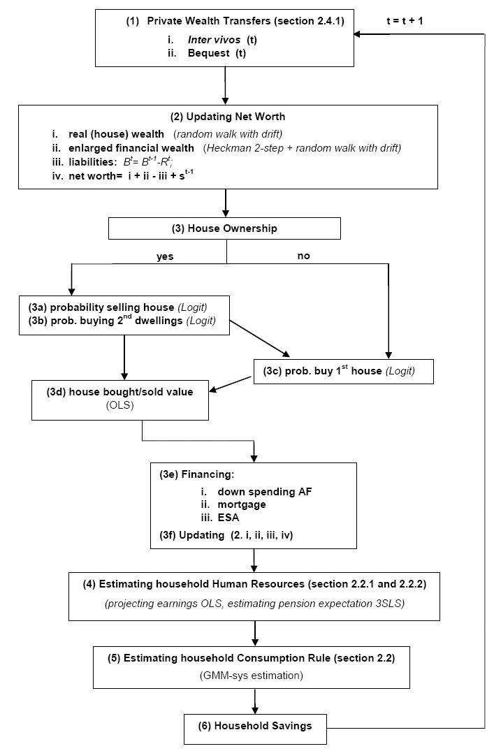
Figure 1 summarizes the sequence of processes for the mechanisms of formation, transmission and spend down of household wealth.

A stylized scheme of formation and transmission of wealth in the wealth module.
The module adopts the traditional recursive logics of DMSMs, including CAPP_DYN. In addition, some of the simulated processes have a dynamic specification themselves and have been estimated on the panel component of SHIW using the lagged dependent variable6 among the covariates. The decision unit for the wealth processes is the household.
For simulation purposes, we adopt a re-coding of SHIW wealth variables into two macro-aggregates: (a) home equity (real wealth) (b) an enlarged financial wealth component, which includes all financial assets plus tangible goods other than real estate (which are assimilated into non-risky assets). Net worth is obtained by subtracting financial debt (if any) from total gross wealth.
As mentioned above, the first simulated events are the intergenerational transfers of wealth between parents and children outside the family of origin (inter vivos and mortis causa). The inter vivos transfers have been modelled by means of a probabilistic approach based on a Heckman two-step procedure in order to account for selection bias. Bequests instead have a mechanical functioning. Due to insufficient information on financial transfers in the SHIW for our purposes, we have used a different micro data source that specifically focuses on this issue: the Survey of Health, Ageing and Retirement in Europe (SHARE). Section 2.4.1 discusses details of the econometrics and the mechanics of this sub-module.
Next, the model updates the wealth stock by assigning a specific return to each asset in order to determine current wealth value (as a random walk with drift based on the mean of the asset return itself). Returns are derived from an iid draw from a specific normal (or Pearson) distribution with constant mean, variance (and kurtosis) derived from available time series for Italy. This step introduces the individual portfolio risk in private accumulation process. The current home equity value of household h, (AHt) is obtained as7
For financial wealth, in order to account for differential returns on the share of risky (φt)8 and non-risky9 assets, we preliminarily estimate financial wealth allocation between these two components with a dynamic model accounting for persistence in attitude toward risk (A static model determines initial conditions for newborn households) and for the role of other observables with a selection model à la Heckman. Since we assume the non risky share of financial wealth accrues a null real return, the weighted rate of return on overall enlarged financial assets amounts to
We assume the borrowing rate – rm – normally distributed with mean and standard deviation to be fixed over time once the mortgage has been taken out and the mortgage repayment to be constant. The net wealth is then given by the sum of real and financial wealth minus the outstanding debt (i.e. mortgages being the only form of borrowing we allow in the model).
In the following step the model simulates choices affecting the stock of real estate and the number of dwellings owned by the family.
The decisions to buy or sell a house work on a set of discrete choice models (logit, estimated on the pooling of 1989–2006 waves of SHIW-HA) combined, in simulation, with Monte Carlo techniques. The totals are then calibrated to match an official external source (ISTAT, 2005). First, the model distinguishes between households that already own at least one house, which are allowed to sell a property, and households that do not have housing equity, which are not allowed to sell.
Once the family is selected for the “sale” event, the value of home equity sold AHst is heuristically assumed to be the current value of real wealth divided by the number of houses owned. The new value of household real wealth is the difference between the current real wealth and the value of the sold house.
The financial wealth is assumed to increase by the value of equity that may exceed the existing debt
Next, a similar procedure applies to purchase of houses. When a household is selected for buying a home, the value of the purchased dwelling (
purchase with down-spending of up to 90% of the enlarged financial wealth; in this case financial wealth decreases by the price of the house bought, real wealth increases by the same amount and any debt does not vary;
if the price of the house exceeds the 90% threshold, the financial advance can be added to by creating new debt for the difference between the house value and the 90% of financial wealth:
; (real and financial wealth are updated accordingly); In Italy, private sector employees receive an additional, and sizeable, severance indemnity at retirement (Trattamento di Fine Rapporto, i.e. end-of-service allowance – henceforth ESA). In practice, the ESA is a deferred share of wage, which can also be partially redeemed in some special cases, and in particular for the purchase of the 1st house or can be fully or partially transferred to complementary pension funds.
Hence, if at least one of the two spouses has an accrued end-of-service allowance (ESA) and the purchase concerns the first house, a 70% redemption of it is allowed as a set-off of debt contracted in ii):
Finally, since the issued debt may be excessively high due to low financial assets relative to the price of the house, we control mortgage sustainability by setting a ceiling to the (total) instalment, as the 40% of the current household net labour and pension income. If the instalment exceeds the threshold, we force the instalment to the ceiling
Subtracting the pre-existing debt from this amount, one obtains the maximum amount that can be loaned in the current period to buy the house:
In the last steps of the loop the model predicts household human lifetime resources, which are the present discounted value of labour incomes stream until retirement plus the pension income flows until household extinction (see Section 2.2.1 and 2.2.2 for details). This aggregate is crucial for determining household consumption expenditure.
This latter cannot exceed the sum of all disposable households income and the “liquid” financial wealth [(1- φt)AF] net of any mortgage installment.
Finally, yearly household savings are obtained as the difference between disposable labour and pension incomes (net of mortgage instalment) and consumption:
The following subsections describe and discuss each sub-module starting, however, from what we conceive as the core of the model, i.e. the consumption rule and the estimation of household lifetime human resources rather than following the order of appearance outlined in Figure 1.
2.2 Household behaviour
In this section we illustrate the theoretical background of modelling households’ behaviour in allocating resources for consumption over different periods of their life. Our aim is to estimate a general consumption rule in order to capture some possible behavioural reactions related to gradual changes in pension outcome expectations as a consequence of a significant social security reform characterized by a long transition phase.
Assuming a homothetic – non-separable over time – utility function, we can derive a closed-form lifecycle consumption function from the optimization problem as elaborated in Modigliani and Brumberg (1954 and 1979). Hence, our general formulation – in order to get an approximate optimizing model – is given by:
s.t.
Where:
a = age of household head
= current consumption = last period consumption for the same household (internal habit) = non-human household wealth in year t when the age of the household head is a = current household disposable income (earnings and pensions) in year t when the age of household head is a π = period constant probability of household extinction
H = household characteristics and type
r = real interest rate
where, in particular, HR represents the (expected) lifetime human resources (or human wealth) given by the discounted future labour and pension incomes stream. The “structural” element of the equation lies in the introduction of expectations about future income stream, through the role of human resources, as a determinant of household consumption.
For the estimation we choose an empirical specification which well describes the consumption/saving behaviour of Italian households in our sample, summarized in the formula:
The implications of such an empirical specification and the econometric estimation will be discussed in Section 2.3.
In the dynamic simulation program, this equation provides us with a predicted value for the current level of consumption
i.e. current household consumption can never exceed the sum of current disposable income plus the liquid share of enlarged financial wealth (non-risky assets), net of the mortgage instalment (if any)
2.2.1 Household lifetime human resources (HR)
In this section we focus on the definition of total household expected human wealth, the estimation of which is preparatory to estimating the consumption rule. The expected value of human wealth is empirically obtained by aggregating spouses’ individual projected (after tax) incomes (earnings and pensions), plus the stream of adult children’s (living within the family) expected labour incomes up to the age of 30, plus one year of earnings contribution of active children over 30.
In algebraic terms:
where:
k = 1,2 adult members
j = active children up to 30 living in the household
= net labour income of household member k (or j) expected in year t when he/she will be aged a+i = net old-age pension benefit of household member k expected in year t when he/she will be aged a+i, or, if already retired, projection of current old age (or survivor) pension benefit in year t when he/she will be aged a+i pk = expected retirement age for spouse k
ak = age of spouse k
Tk = expected death age for spouse k (according to ISTAT projections)
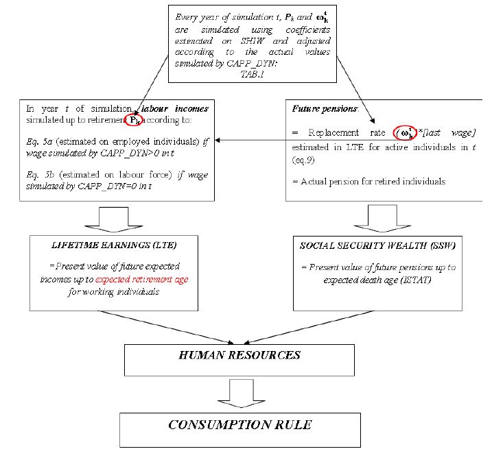
Therefore, in order to evaluate this (stock) variable we need to evaluate its three main components, i.e. household lifetime labour income, expected social security wealth for active individuals and current (residual) social security wealth for the individuals who are already retired. It is worth noting that, in the simulation program, the predicted values of estimated equations used to build HR are re-computed every year – using current simulated values of explanatory variables – so as to obtain the current value of HR which, in turn, is a determinant of the yearly simulated consumption.
Individual projected lifetime income profiles
Individual lifetime earnings are defined as the present discounted value of future expected labour income flows up to the planned age of retirement. The projection in t for income at time t+i (where i is a generic period between t – current year – and the age of retirement (pk – t)) for each individual k or j is obtained as the prediction of the following econometric models where age is ak+i:
or
where ln
We use two models estimated on the 1989–2008 panel component of SHIW to obtain a projection of labour income until retirement.
In particular, we use a dynamic specification to estimate the process to be simulated when the individual has a positive wage in the current period (which represents the lagged variable for predicting the expected wage for the following year) (5a), while we use a static specification fitted on both employed and unemployed individuals for active individuals with zero wage in t, e.g. in the case of unemployment (5b).
Hence, the present value of the expected labour income at a generic age a+i,
where the (1+g) factor allows the wage level to be linked to the (five-years MA) medium-long run productivity growth which is calibrated through the “Scenario” block of the pre-existing CAPP_DYN modules, and β and δ represent the discount factor according to a quasi-hyperbolic time preference13.
Finally, in order to obtain individual lifetime income, we need to sum the present value of the projected labour incomes for every t from the current period up to the expected retirement age pk. However, pk is not known a priori either12.
Indeed, pk, along with the expected replacement rate
Planned retirement age and (related) expected replacement rate
Reforms implemented in Italy from 1992 to 2007 have significantly affected the institutional social security framework, introducing a tight actuarial link between contributions paid and pension received back. As a consequence, the long term financial sustainability of the social security system will be assured, though the expected replacement ratio for future pensioners is expected to fall.
These new computational rules will affect incentives to retire. While for those whose pension is calculated with the old defined benefit (DB) formula the expected retirement age can be reasonably expected to match the legal provision (or the age at which individuals accrue the seniority requirements), for workers instead falling under the mixed and, especially, under the notional defined contribution (NDC) regime, the expected retirement age presents substantial challenges. We need to model the behaviour of individuals who will have to face very different scenarios and will therefore not be able to draw from the experience of previous generations.
Since we consider subjective expectations to matter in economic decisions, we use the expected replacement rate and the planned retirement age information reported in the SHIW13 survey and we build an econometric model for imputing out-of-sample values. Data support the hypothesis of an increase in the expected retirement age and a decrease in the expectations on future replacement rates if we consider recent survey waves, suggesting a partial internalization of the effect of pension reforms in the process of expectations-formation.
Since the planned retirement age (PRA) and the expected replacement rate (ERR) are slightly negatively correlated (ρ= −.14) but part of their variability may be jointly determined, there is a strong likelihood that there will be a correlation between PRA and the error term in the model of expected replacement rate (ERR). In order to better account for this kind of endogeneity we then choose to fit a three-stage estimation for systems of simultaneous equations, since PRA is simultaneously the dependent of the first equation and an explanatory variable in the second equation (ERR) of the system.
With regard to the first equation of the system (Table 1), i.e. the planned age of retirement, we can notice the contributive seniority (and its square) has a negative coefficient, while in order to account for the role of age and its correlation we interact the latter with the former. Then, we could be tempted to interpret its positive and significant coefficient as a counter-effect of age (perhaps due to an adjustment of individuals’ planning when they approach to retirement), given the expected negative impact of seniority. In practice, age and seniority cannot be separately identified, this strategy allowing only the feasibility of estimation, but not the interpretation of coefficients as causal effects.
Three-stage least-squares regression of planned age of retirement and the expected replacement rate.
| Equation | Obs | Parms | RMSE | R-sq | chi2 | P | |||
|---|---|---|---|---|---|---|---|---|---|
| 1. PRA | 27194 | 21 | 3.435451 | 0.257 | 9408.45 | 0 | |||
| 2. ERR | 27194 | 21 | 0.163388 | 0.149 | 5043.9 | 0 | |||
| Planned Age of Retirement | Expected Replacement Rate | ||||||||
| B | SE | B | Se | ||||||
| year_contrib | −0.5187 *** | 0.0138 | PRA | 0.0026 ** | 0.0010 | ||||
| year_contrib² | −0.0093 *** | 0.0003 | year_contrib | 0.0064 *** | 0.0009 | ||||
| age*contrib. | 0.0148 *** | 0.0003 | age*contrib | 0.0000 | 0.0000 | ||||
| female | −2.0137 *** | 0.0523 | NDC | −0.0292 | 0.0180 | ||||
| NDC | 0.1496 | 0.3824 | single | −0.0024 | 0.0050 | ||||
| Education (omit.lower secondary) | |||||||||
| upper_secondary | 0.2877 *** | 0.0557 | upper secondary | 0.0130 *** | 0.0026 | ||||
| degree_or_more | 0.8929 *** | 0.0842 | degree or more | 0.0094 * | 0.0040 | ||||
| self_employed | 1.2709 *** | 0.0646 | self employed | −0.1168 *** | 0.0033 | ||||
| public | −0.2373 *** | 0.0632 | public | 0.0457 *** | 0.0030 | ||||
| home_owner | −0.1369 * | 0.0564 | partime | −0.0363 *** | 0.0047 | ||||
| South | 0.6384 *** | 0.0580 | Centre | 0.0321 *** | 0.0030 | ||||
| single | 0.3774 *** | 0.1072 | South | 0.0427 *** | 0.0030 | ||||
| tau2002 | 0.0625 | 0.0751 | tau2002 | −0.0298 *** | 0.0035 | ||||
| tau2004 | 0.2979 *** | 0.0774 | tau2004 | −0.0453 *** | 0.0036 | ||||
| tau2006 | 0.0922 | 0.0805 | tau2006 | −0.0739 *** | 0.0037 | ||||
| tau2008 | 0.8402 *** | 0.0978 | tau2008 | −0.0793 *** | 0.0047 | ||||
| Cohort effect (omit. Cohorts <1953) | |||||||||
| coor_53 | 1.1369 *** | 0.1010 | coor_53 | 0.0122 ** | 0.0046 | ||||
| coor_58 | 2.0562 *** | 0.1234 | coor_58 | 0.0165 ** | 0.0056 | ||||
| coor_63 | 2.5093 *** | 0.1462 | coor_63 | 0.0257 *** | 0.0065 | ||||
| coor_68 | 2.5112 *** | 0.1672 | coor_68 | 0.0393 *** | 0.0071 | ||||
| coor-73 | 2.3387 *** | 0.1844 | coor-73 | 0.0660 *** | 0.0075 | ||||
| coor_78 | 2.0769 *** | 0.2041 | coor_78 | 0.0688 *** | 0.0081 | ||||
| intercept | 61.3483 *** | 0.1937 | intercept | 0.4269 *** | 0.0635 | ||||
| Endogenous variables: PRA, ERR | |||||||||
-
*
p<.05.
-
**
p<.01.
-
***
p<.001.
-
Source: Authors’ computations on SHIW 2000–2008.
Time dummies (tau) catch the slight extension in planned retirement in the more recent waves, while cohort dummies (coor) do not suggest a clear-cut pattern apart from the fact that individuals born after 1953 plan to retire later than older individuals.
Looking at the second equation, the expected replacement rate, we can see how the simultaneous estimation corrects the endogeneity of planned retirement age as a regressor by estimating a positive, significant, coefficient; the contributive seniority, as expected, has a positive impact while its interaction with age has a null effect. Individuals falling under the NDC pension scheme expect, on average, 3 points less in their future replacement rate but, once controlling for all other covariates, the effect does not seem to be significantly different from zero. Also in this equation, but with a clearer pattern, time dummies catch the recent (downward) revision in pension outcome expectations, while cohort dummies surprisingly show, other things being equal, that the younger the cohort the higher the expectation about future replacement rate. Once again, time, cohort and age effects are only identified by functional form in these models and causal effects are hard to be interpreted.
In the light of this empirical analysis, since the expectations-adjustment process is not fully completed, it would be unreasonable to assume that pension expectations will remain unchanged in the future. On the opposite, these expectations will become increasingly accurate over time.
Therefore, the projected values for these two variables pk and
The weight of this average ∈ (0,1) becomes closer to zero the closer the year of simulation is to 2050 (i.e. the more the pension outcomes of the new NDC regime become observable) and the closer the worker is to his/her retirement age (the closer one is to her retirement age, the more aware he/she is about the exact timing of retirement and about the expected pension amount).
Although actual simulated future values are exogenous to the wealth module (at the state of the art feedbacks from this latter to the former modules are not allowed yet), the social security module of CAPP_DYN – following a rule of exit essentially playing along with the increase in the legal provision – provides an evaluation of the pension benefit that is consistent with a given seniority and with the computational rules related to the particular pension scheme an individual falls under. In other words, we assume that, given a simulated labour market exit-age which only partially reacts to offset the future decreasing pension coverage, expectations about the implied replacement rate should converge towards its actual value.
2.2.2 Social security wealth
In order to estimate the expected value of future pension benefits, the model computes the expected value of the first annuity by multiplying the estimated expected replacement rate
The expected present value of future pension flows is obtained as the sum of present values of pension annuities from retirement to the expected age of death (Tk,a+i) (calibrated according to ISTAT projections depending on age, gender and year):
where Pk,i is the projected pension for active individuals, and actual simulated pension for retired individuals.
Finally, SSW values are further discounted back to the current period with the βδ1 quasi-hyperbolic discount factor used for lifetime earnings projections and aggregated for the spouses. By summing the life-time labour incomes component plus the pension component, the model produces an estimate of the expected value of household human resources (HR).

Estimation and simulation of human resources.
2.3 Estimation of the consumption rule
In this section we discuss the specification and the estimation of the consumption rule, whose parameters are used in the simulation program. As mentioned in the introduction, the idea driving our approach is that the likely impact of structural social security reforms on the consumption/savings age profile of Italian households asks for a step beyond the estimation of a traditional reduced-form Keynesian equation. In fact, looking at the recent past (i.e. our 1989–2008 panel dataset, Figure 3), we notice that the saving propensity profile of Italian households is characterized by a nearly flat pattern from about 35 years on, with pensioners having, on average, a positive propensity to save even at older ages.

Average equivalent consumption (left) and propensity to save (right) household-head-age-profile.
A broad strand of literature has investigated the so called “retirement consumption puzzle” in several countries (Lundberg et al. 2001, Fernandez and Krueger, 2004). For Italy, some authors have explained – at least partially – the high (private) savings propensity of the elderly by the generosity of the social security system (Miniaci et. al, 2003) which, so far, provided pensioners with rather high rate of returns on contributions and high replacement rates. Once social security wealth is included in the total wealth, the savings profile of Italian households turns out to be more consistent with the lifecycle hypothesis, with a positive propensity until retirement and a spend-down phase in the ensuing period14.
We believe that taking this pattern as given and projecting it into the forthcoming decades – when social security reforms will be fully operational and the generosity of public pensions will be much reduced – would result in missing an important part of the distributional story. In fact, reform especially affects the current young and future workers whose lifecycle consumption is not (or only incompletely) observed and whose expectations have only partially embodied the long-run effects of the reforms themselves. We therefore believe that linking consumption behaviour to a lifecycle theoretical framework, searching for a specification that fits our data more closely, is an appropriate strategy for accounting for such issues. This topic will be further addressed in Section 3.
As mentioned in Section 2.2, the empirical specification is the following:
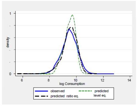
Such a functional form, where the dependent variable is (the log of the) consumption to HR ratio, proves to better fit our household consumption data across the distribution (which is an attractive feature in a micro simulation distributional model; see Figure 4) at the same time considering the role of habit persistence and the effects of future expectations about incomes and pension outcomes as crucial determinants of current consumption. Moreover, by estimating a propensity rather than a level, in the simulation program we get rid of the necessity to make arbitrary assumptions on dynamics of aggregate consumption due to its non-stationarity in a dynamic economy. In other words, if we simulated in levels, we would need to align consumption in addition to income. On the opposite, we would like consumption to be an endogenous outcome of the model, with respect both to its variance and to the mean itself (i.e. no alignment).

Post-estimation predicted consumption from dynamic model in level vs ratio.
In order to estimate the dynamic consumption function (10) we use a GMM system estimator (Arellano, Bover, 1995; Blundell, Bond, 1998) with robust standard errors so as to purge the estimations from the bias induced by the endogeneity due to the individual fixed effect.
A consequence of the periodicity of the survey is that the reference consumption propensity is the two-year lag causing a weaker estimated persistence parameter (Lag.ln{C/HR} =0.082) when implemented in the discrete yearly simulation program.
Both the (log of) enlarged financial wealth (af_en) and financial debt (pf) have positive elasticities on the propensity to consume out of human resources while housing equity (ar_h) shows a negative elasticity. This latter, however, has to be evaluated in the light of the interaction with the number of owned dwellings. The positive sign of the interaction coefficient probably indicates a non-linear effect of real wealth on the dependent variable as owners of more than one property often enjoy actual rents (besides imputed rents for owner-occupied dwellings) that represent an extra-source of (capital) income which can be allocated to consumption.
The negative effect of retired household head (hh_retired)15 confirms the well-known drop in consumption at the time of retirement. Moreover, the household residual life (h_res_life), determined according to the survivor probabilities of the youngest spouses, determines a drop in the consumption propensity. Finally, the effect of household types suggests that nuclear families, i.e. couple with or without non-working children – the reference (omitted) category – are characterized by a lower propensity to consume out of the human life-time resources.
Dynamic panel-data estimation of the consumption rule, two-step system GMM 16.
| ln{C/HR} | B | Se |
|---|---|---|
| Lag.ln{C/HR} | 0.0821 *** | 0.0209 |
| In_af_en | 0.0114 *** | 0.0024 |
| In_ar_h | −0.0171 *** | 0.0014 |
| In_ar_h*n_houses | 0.0040 *** | 0.0006 |
| In_pf | 0.0092 *** | 0.0012 |
| quintile 2_income | −0.1347 *** | 0.0181 |
| quintile 3_income | −0.1832 *** | 0.0206 |
| quintile 4_income | −0.2559 *** | 0.0232 |
| quintile 5_income | −0.3105 *** | 0.0272 |
| hh_age | −0.2152 *** | 0.0491 |
| hh_age² | 0.0066 *** | 0.0013 |
| hh_age³ | −0.0001 *** | 0.0000 |
| hh_age4 | 0.0000 *** | 0.0000 |
| hh_age_self_emp | −0.0026 *** | 0.0004 |
| hh_age_upper_secondary | −0.0009 *** | 0.0002 |
| hh_age_degree_or_more | −0.0032 *** | 0.0004 |
| h_res_life | −0.0143 *** | 0.0027 |
| hh_retired | −0.1282 *** | 0.0213 |
| earners_ratio | −0.2058 *** | 0.0326 |
| n_child_in the family | 0.0232 ** | 0.0087 |
| South | −0.0489 *** | 0.0109 |
| Household types (omitt. Nuclear family) | ||
| Single | 0.0108 | 0.0211 |
| nuclear single headed | 0.1754 *** | 0.0356 |
| non_nuclear single headed | 0.4704 *** | 0.0350 |
| non_nuclear | 0.1948 *** | 0.0174 |
| Time dummies (omit.tau2002) | ||
| tau1993 | 0.0148 | 0.0191 |
| tau1995 | 0.0623 ** | 0.0193 |
| tau1998 | −0.0699 *** | 0.0210 |
| tau2000 | −0.4194 *** | 0.0194 |
| tau2004 | −0.0219 | 0.0176 |
| tau2006 | 0.0228 | 0.0186 |
| tau2008 | 0.0018 | 0.0182 |
| intercept | −0.2847 | 0.6923 |
-
N = 23,426, number of groups = 10,284.
-
Arellano-Bond test for AR(1) in first differences: z = −18.00 Pr > z = 0.000.
-
Arellano-Bond test for AR(2) in first differences: z = 0.49 Pr > z = 0.627.
-
Sargan test of overid. restrictions: chi2(7) = 7.60 Prob > chi2 = 0.369.
-
Hansen test of overid. restrictions: chi2(7) = 4.79 Prob > chi2 = 0.685.
-
Difference-in-Hansen tests of exogeneity of instrument subsets:
-
GMM instruments for levels.
-
Hansen test excluding group: chi2(6) = 4.60 Prob > chi2 = 0.596.
-
Difference (null H = exogenous): chi2(1) = 0.20 Prob > chi2 = 0.658.
-
*
p<.05.
-
**
p<.01.
-
***
p<.001.
-
Source: Authors’ computations on SHIW data, Historical Archive, panel component, waves 1991–2008.
2.4 The intergenerational transfers sub-module
This section describes the functioning of another important block of the Wealth module. This part of the model proves to be of fundamental importance in modelling private wealth within a dynamic microsimulation framework aimed at explicitly accounting – in a probabilistic fashion -for inter-generational links and at assessing the between/cohorts role of private wealth transmission. From a micro perspective, intergenerational transfers may reduce inequality between cohorts but may conversely also increase economic disparities within cohorts. Either way, they may be an important channel for transmitting economic inequalities.
The analysis of such phenomena plays an important role in our study both as the size of the wealth transfers is not negligible, and because intergenerational transfers may support or even substitute for social security transfers, especially when the latter will play a decreasing role in the future. The question is even more crucial when considering three main features of Italy’s demography and economy: the secular decline in fertility, which is greater than in other European countries; the high saving rate of the elderly; the mortgage market imperfections which, causing big borrowing constraints for the young, would even further reduce their consumption capabilities and the possibility to buy a home without substantial private wealth transmission.
Concerning the quantitative evaluation of such a phenomenon, data available for Italy are still narrow. The only two sources are the Bank of Italy’s Survey on Household Income and Wealth (SHIW, 1992 and 2002 waves) and the Survey of Health, Ageing and Retirement in Europe (SHARE), which collects information on a representative sample of individuals over 50. This survey collects richer and more detailed information on wealth intergenerational transfers (and time in the form of reciprocal care) compared with SHIW and allows cross country comparisons. This micro data source has the unusual feature of collecting detailed information on respondents’ children living out of the family of origin, allowing a donor-recipient matching very useful in analyzing determinants of intergenerational transfers.
2.4.1 Implementation of the transfers sub-module in CAPP_DYN
In this section we describe the structure of the intergenerational transfer sub-module of CAPP_DYN. This module includes the set of procedures which allow the transmission of financial and real wealth (this latter only in bequest processes) among family units in every year of simulation.
In the simulation program, wealth transfers may occur inter vivos or mortis causa. The former involves redistribution of wealth from donor to recipient families during their life cycle. The latter occurs when a household extinguishes in the model (because all of its members died), through the distribution of net wealth (whether positive) among heirs.
In the current release of the model we assume that the inter vivos transfer decisions depend on socio-economic characteristics of the observational unit. In other words, first the model determines such characteristics within the original blocks then, conditional to these observables, wealth transfers are simulated. Therefore feedbacks from wealth decisions to demographic, occupational and pension choices are not allowed yet. The methodology we adopt in the inter vivos estimates is based on a traditional two part approach with Heckman correction in the OLS estimation of the amount, whether it is needed.
We model separately the two sides of the transfer (donor and recipient). We do not model this process as a simultaneous choice due to a higher share of out-of-sample families in the first years of simulation that does not allow to treat the initial sample as the real population. For this purpose, we build two datasets: the original, which we call “potential donors,” and the derived one, which we call “potential recipients” (where units are child’s families). We then estimate the two sides of the exchange separately on the two datasets using some mutual characteristics (i.e. recipients characteristic in the donor equation and vice versa). The inclusion of such characteristics in the equations (especially, the parents’ financial wealth in the recipient regression) allows us to explain a quite similar share of the variance of the dependent variables in the two outcome equations (i.e. transfers given and received), providing predicted values characterized by similar variability. This property proves to be important in the simulation stage in order to avoid excessive under-estimation of the intergenerational transmission of inequality through an unrealistic within cohort redistributive effect of private wealth inter-generational transfers.
The sub-module is structured as follows: among households with head aged over 50 and with a positive wealth in the previous period, the model selects those with the highest transfer probability employing a binary variable that is equal to 1 if the interviewed household has made at least one transfer towards children or grandchildren in the 12 months preceding the interview, 0 otherwise. For the outcome equation the dependent is built as the logarithm of the transferred amount on donor financial wealth17 (gross of transfer) ratio.
Once donor households have been identified and the amount of transfer has been determined, the down spending of donors’ wealth is deterministically simulated by subtracting the amount transferred by the pre-transfer held stocks.
For the recipient model, the dependent variable is a binary that is equal to 1 if the observed child’s household received a transfer in the 12 months preceding the interview, while in the outcome equation the dependent variable is the logarithm of the transfer received.
Among the covariates of the recipient model, besides a polynomial in age we use some occupational and household structure controls plus the existence of children (named Grandchildren, for the donor) and the (pre-transfer) financial wealth of the family of origin [ln(af parents)].
In the Tables 3 and 4 we report estimated coefficients for the two separate models.
Two-step estimation for intergenerational giving with Heckman correction.
| Donor side N=16,871 | |||||
|---|---|---|---|---|---|
| Logit Probability of being Donor | OLS ln{Ratio} | ||||
| B | Se | B | Se | ||
| age | 0.0807 *** | 0.0243 | age | −0.7785 ** | 0.2404 |
| age2 | −0.0007 *** | 0.0002 | age2 | 0.0113 ** | 0.0036 |
| in_work | 0.3522 *** | 0.052 | age3 | −0.0001 ** | 0.000 |
| quintile 3_wealth | 0.4146 *** | 0.0543 | in work | −0.4384 *** | 0.0866 |
| quintile 4_wealth | 0.6046 *** | 0.0531 | retired | −0.2449 ** | 0.0849 |
| quintile 5_wealth | 0.6989 *** | 0.0531 | unemp | −0.4619 ** | 0.1649 |
| child_unemp | 0.2835 *** | 0.0625 | ch_unemp | 0.3006 *** | 0.0817 |
| wed_or_birth | 3.2668 *** | 0.1205 | quintile 3_wealth | −0.5422 *** | 0.0752 |
| upper_secondary | 0.5074 *** | 0.0463 | quintile 4_wealth | −0.8931 *** | 0.0736 |
| degree_or_more | 0.742 *** | 0.0502 | quintile 5_wealth | −1.4278 *** | 0.0733 |
| Italy | −0.2737 *** | 0.0747 | Italy | 0.7029 *** | 0.0951 |
| _intercept | −4.4368 *** | 0.8158 | mills_ratio | 0.2653 *** | 0.0414 |
| _intercept | 15.5409 ** | 5.3305 | |||
-
T
-
*
p<.05.
-
**
p<.01.
-
***
p<.001.
-
Source: Authors’ computations on SHARE data, wave 2004.
Two-step estimation for intergenerational receiving without Heckman correction.
| Recipient side | |||||
|---|---|---|---|---|---|
| N=29,652 Logit Probability of being Recipient | N= 1,872 OLS ln{Amount} | ||||
| B | t | B | Se | ||
| In(af parents) | 0.169 *** | 0.061 | In(af parents) | 0.0892 *** | 0.0079 |
| age | −0.0883 *** | 0.052 | age | 0.0253 * | 0.0147 |
| age² | 0.0007 *** | 0.0543 | age² | −0.0004 * | 0.0002 |
| married | 0.3004 ** | 0.0531 | grandchildren | −0.1051 * | 0.0567 |
| single | 0.6497 *** | 0.0531 | married | 0.1911 *** | 0.0494 |
| divorced | 0.6462 *** | 0.0625 | Italy | 0.2481 ** | 0.0944 |
| in work | −0.2689 *** | 0.1205 | _intercept | 7.028 *** | 0.2699 |
| degree | 0.3421 *** | 0.0463 | |||
| grandchildren | 0.2863 *** | 0.0502 | |||
| Italy | 0.1984 ** | 0.0747 | |||
| _intercept | −1.3815 *** | 0.8158 | |||
-
T
-
*
p<.05.
-
**
p<.01.
-
***
p<.001.
-
Source: Authors’ computations on SHARE data, wave 2004.
For the donors model, the evidence shows a lower probability joint to a larger share of transferred wealth for Italian households.
Belonging to higher net wealth quintiles still has a positive sign in the logit, but has a negative sign in the outcome equation. Therefore, the better-off households show a higher transfer probability but, as a share of their financial wealth, they transfer less compared to less-affluent families. Moving on to the recipients’ characteristics, the determinant role of some specific events in the recipients’ lives (such as unemployment – child_unempl -, marriage, childbirth – wed_or_birth) is confirmed and increases both the probability to be donors and the amount. In particular, the latter variable, i.e. wed_or_birth, is strongly significant and very powerful (coefficient 3.2) in predicting the financial giving event.
Turning to the recipient equations (Table 4), due to the derived nature of the dataset, we can estimate only a model with a reduced number of covariates and no valid exclusion restrictions. Italian recipients show both a higher average probability and a greater average amount compared to the other European counterparts. This evidence seems at odds with the lower giving probability in the Table 3. Nevertheless, Italian households tend to transfer more often to all of their children and have, on average, a slightly few number of children compared to the overall sample. Finally, a powerful determinant of transfer receiving is, as expected, the financial wealth of the family of origin
The (log) value of parents’ financial assets for family units without a potential donor in the sample in a period t is obtained as a draw from a normal distribution with mean and variance equal to the actual first and second moments of the financial wealth distribution among over 50 families in period t. This procedure implicitly assumes that the future distribution of financial wealth will change in its mean and variance only (not a very strong assumption) and that such a draw is independently distributed over time18 and across families. We follow this approach rather than simply excluding this variable from the set of recipient equations regressors, in order to warrant an acceptably good match between the variances of given and received simulated transfers19.
Next, the model verifies the consistency between the total (out-and-in) flows and, every year, imposes the following condition by alignment:
Where J and K are households giving (G) and receiving (R) a transfer, respectively, while af is the amount of transferred financial wealth. Condition (11) ensures an accounting consistency in the process of inter vivos transmission.
Should a family unit extinguish due to the death of the last remaining member, the model simulates the (proportional) transmission of the whole wealth endowment to the heirs. To this end, we try to account for the main family relationships in order to define the heirs’ share of bequests. Currently, CAPP_DYN allows considering relationships among individuals who, during the survey (2002), shared the same house, and those living outside the family of origin at that time. We consider therefore as potential heirs all the children, grandchildren and common-law spouses in the initial population plus the children living outside (i.e. not included in the sample) plus those born during the simulation period.
Once the number of heirs’ families is defined, bequests are deterministically simulated with the stock of wealth being proportionally distributed among them in the form of financial wealth. Then, in order to ensure the accounting consistency of the wealth stocks in the economy, every year the model imposes the following identity:
where J is the number of extinguishing family units in each year that pass on their wealth (G) mortis causa, K is the number of in-sample heirs that receive a bequest (R), nw is the net wealth transferred amount (in the form of financial wealth) and Res is the residual amount consisting of the net wealth of households which have extinguished without heirs plus the wealth shares received by out-of-sample heirs.
This latter residual has been imputed through calibration; therefore Res has been distributed as a proportion of net worth already held by the household, in order not to alter the sample wealth distribution.
3. Simulation results
In this section we present some selected simulation results provided by the extended version of CAPP_DYN including the new Wealth module. In particular, our aim is to compare our semi-structural life cycle approach (LC) with an alternative non-structural framework (NS), based on the estimation and the projection of a simple Keynesian consumption function enriched with socio-demographic and wealth covariates (i.e. consumption not depending on life cycle resources).
There are two main reasons why we adopted a semi-structural modeling of consumption behavior. The first one grounds on a theoretical rationale. Using a Keynesian consumption equation, one implicitly assumes the structure of the propensity to consume current income remaining invariant to radical institutional changes. This would imply replicating in the long-run an inverted U-shaped consumption, with a sharp decline after retirement and a quasi-flat propensity to save profiles, as those observed on actual survey data20 (Figure 3).
However, next future will be characterized by two significant transitions – in the demographic structure (particularly pronounced in Italy) and in the public pension system, which will slowly shift from quite a generous (though horizontally unfair) defined benefit system (DB) to an actuarially neutral notional defined contribution regime (NDC). The gradual social security reforms are expected to place most of the burden on current young (and future) workers through a significant cut in their expected returns on social security contributions. In addition, demographic changes will bring a large increase in the population share of elderly; on the other hand, older cohorts – characterized by a large number of individuals (baby-boom generations), a high net saving rate (despite the generous pension system) and a low number of descendants – will be replaced by later cohorts, less numerous and not enjoying the same social security arrangement. Nevertheless, on average, they would be able to benefit from larger intergenerational transfers of private wealth.
All these changes make the current consumption and saving behavior unsuitable to be regarded as a ‘steady state’ to be projected in the future. Thus, we recognize a semi-structural approach as more appropriate in order to shed light on the likely distributional consequences of transitions.
In the following sections we present some simulation results for the period (2008–2050) starting from a look to the general trends of household propensity to save in order to check their consistency with the model hypotheses. We then focus on the evolution of private intergenerational transfers (inter vivos and bequests). Dynamic MSM endowed with a wealth module allows a more comprehensive examination of distributional dynamics, especially in a long-term intergenerational perspective. Hence, we carry out analyses on net wealth and disposable incomes and their drivers by computing the contributions to the variation in Gini exerted by factors at work in the model.
Table A.1 in the Appendix summarizes all relevant exogenous parameters used in the analysis and reports the different assumptions of two alternative returns scenarios. Whether not differently specified, results are presented according to the LC approach and to the assumptions of the benchmark scenario on returns.
3.1 Aggregate trends
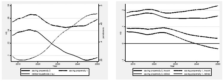
In order to get a macroeconomic picture of the saving patterns simulated by the model, Figure 5 displays aggregate results in terms of propensity to save out of base income (Y0). In particular, two definitions of savings are adopted: s0, the liquid savings (i.e. base income minus consumption minus the mortgage instalment, if any), and s1, obtained by considering the capital share of mortgage instalment as a form of savings (i.e. base income minus consumption minus annual mortgage interest, if any). As it can be noticed, in a first period, up to nearly 2020, the saving propensity increases, followed by a long period of moderation (more dramatic for the s0 propensity).

Average saving propensity (left), propensity to save for active households vs. for retired households (right), 2008–2050.
We can identify some forces driving such pattern. Figure 5 (left panel) also plots the share of households whose head is retired. A sharp increase is recorded in this value, which increases from 35% of the population in 2012 to about 47% in 2045. This could be interpreted as first macro-level determinant of the retrenchment of savings in the second spell if we think of retired people in the future decades behaving differently from current Italian pensioners (who are still net savers at the older ages, see Figure 3).
Indeed, given the behavioural hypotheses introduced in the model, households’ life cycle savings patterns will change, presenting features that were missing in the recent past, thus characterized by greater saving just before retirement and more dis-saving after retirement.
These remarks are made explicit by Figure 5 (right panel) which depicts the evolution of saving propensities for households whose head is working, and for households whose head has retired. A clearly diverging pattern can be observed between the two groups. On the other hand, pension expectations are an important parameter of the consumption rule and their evolution determines the initial upward trend in the propensity to save of active households.
Therefore, so far, we have identified two opposite forces affecting saving pattern in the next years. One is a pro-saving effect due to the internalization of expectations of pension reforms by active people; the other is a counter effect – due to the interaction of future pension outcomes with the life-cycle consumption rule – on the behavior of future pensioners, who are expected to become more dis-savers.
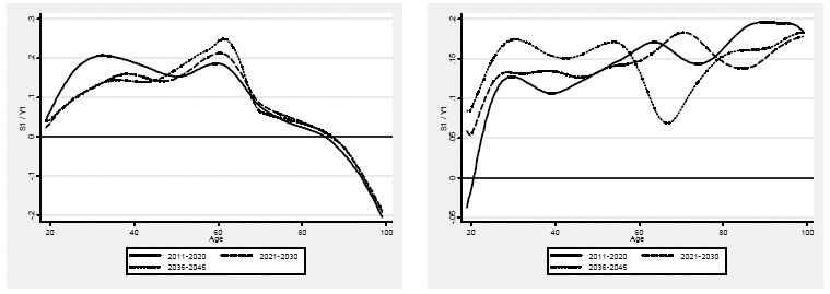
Figure 6 shows the average simulated propensity to save age-profile in the two frameworks – LC vs. NS – in three key periods (2012–2020, 2021–2030 and 2036–2045). As it can be noticed, the NS approach tends to reproduce the past average pattern, implying an anomalous flat or moderately-growing profile even after retirement, still consistent with the retirement consumption puzzle particularly marked so far in Italy (right panel). However, this peculiar evidence can be explained by the presence of a pronounced precautionary savings motive (Jappelli et al., 2006; Lusardi, 1997) and a low consumption propensity of elderly, which, despite the generous pension system, reflects a well-rooted habit persistence (Baldini et al., 2002). In fact, although the earning-related Pay-go social security system, introduced in the 1970s, could have produced a ‘free lunch effect’ in the early cohorts of pensioners, increasing their consumption, the parsimonious preference structure of such cohorts, which were active during or just after the WWII, has prevailed on the former effect.

Propensity to save by age, LC (left) vs. NS (right) simulation, 2011–2020, 2021–2030, 2036–2045 (averages).
Source: Authors’ computations on simulation results.
The second approach displays, on the opposite, a reversal of the above-mentioned profile21, which seems more in line with the experience of other western countries.
We conceive this latter scenario as more conceivable in the future due to a significant reduction in future returns on social contributions introduced by the reforms. In addition, radical changes in the socio-institutional environment such as a severe delay both in entry into a stable occupation and child-bearing, are likely to affect individuals’/households’ future life-cycle consumption-savings profiles too. Finally, the habit persistence itself can play a role, as younger cohorts have embodied a significantly higher living standard. Possible reactions in consumption decision can be bounded, but we account for liquidity constraints in determining simulated consumption (see formula 3).
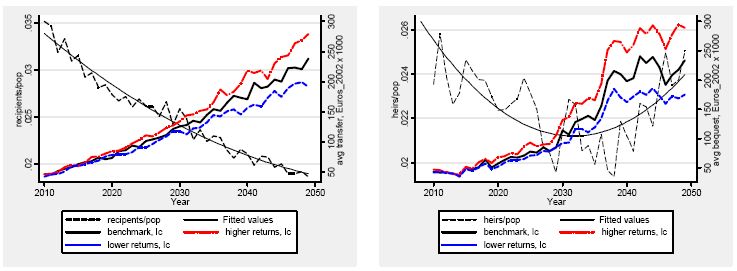
In sum, we conclude the consumption function estimated in the NS approach is hardly conceivable as a steady state relationship Next, we analyze the predicted evolution of private wealth received as a gift or bequest. Figure 7 displays the evolution of the share of recipient families of inter vivos (left) and mortis causa transfers (right) and of the average amount transferred. The share of recipient households decreases from 3.5% in 2008 to 2% in 2050 while the average transfers increases from about 25,000 Euros in 2008 to 240,000 in 2050 (Euros at 2002 prices), according to the benchmark scenario.

Evolution of iv and mc transfers recipient households’ share and of the average amount received, 2010–2050.
Source: Authors’ computations on simulation results (2008–2050).
Considering the product of the two dimensions, the mass transferred inter vivos is expected to grow by a factor five in real terms over the next four decades while the mean wage is expected to double in the same period.
Concerning the private wealth transferred mortis causa, the share of heirs’ families in the population is fairly stable between 2% and 2.5%, while the evolution of the average bequest received can be divided into three sub-periods: a steady and consistent growth from 2010 to 2029, an explosion from 2029 to 2042 and, finally, a third period up to 2050, where the amount remains roughly flat.
Multiplying the average amount by the share of population we get a mass of wealth bequeathed in 2050 equal to more than five times the one of 2008.
In terms of average growth, both for inter vivos transfers and bequests, throughout the simulation period the model predicts a noteworthy compound annual growth rate of about 4% (with an acceleration in the central period, i.e. the time when the baby-boom generation is expected to pass away), well above the general growth in wages. Such growth rate is reduced to 3.3% in the low return scenario while it is boosted to more than 4.5% according to the high returns assumptions.
This evidence points out a non-negligible role the intergenerational transmission of private wealth is going to play in the coming decades, both in the dynamics of household accumulation and in wealth distribution, due to its high dispersion.
3.2 Distributional results
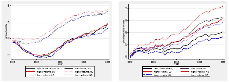
This section aims at exploring the distributional implications of results provided by our simulations. Figure 8 below depicts the overall evolution in the Gini of projected net wealth among Italian households (left) as well as of equivalent disposable income (Y2) obtained by summing net labour and pension incomes (Y0) with annual rents provided by home equity (net of interests on mortgage, if any), and income from enlarged financial wealth22 (right). The results are plotted both across the two behavioral approaches (LC vs NS) and the three returns scenarios. Difference between thin and thick lines in the figures can be thought of as ‘second order’ effects of assuming a life cycle savings, curbing (yet not reversing) the tendential surge of wealth and disposable income inequality. Although the distributional consequences of a life-cycle consumption structure are minor relative to the first order effects, the impact is not negligible.

Evolution in the Gini of net worth (left) and disposable income (right), 2010–2050.
Source: Authors’ elaboration on simulation results.
Concerning dynamics, according to the LC approach net wealth inequality is expected to decrease by roughly 38 basis points until about 2025; after that the model predicts a sharp increase in Gini.
Inequality in equivalent overall disposable income is expected to progressively increase all over the simulation period.
As it can be noticed, while assumptions on average returns are roughly neutral in terms of wealth inequality dynamics, whose range of variation among scenarios on returns appears rather thin, they exert a dramatic influence on disposable income. Considering jointly different scenarios on returns and behavioural approaches, at the end of the simulation period the difference in Gini between low returns LC and high returns scenarios NS (lower and upper bounds, respectively) stands to about 60 basis points
The analysis of the contributions of each wealth component in shaping inequality is a specific task of the Wealth module. In order to better disentangle the role of different ‘accumulation channels’, we compute the contributions to variation (i.e. the first difference) in Gini of wealth exerted by the factors at work in the model: intergenerational transfers, savings, capital gains and end-of-service allowance.
In fact, wealth (W) can be conceived as the sum of lagged wealth and current severance indemnity (ESA), savings (S), received net of given transfers (inter vivos and mortis causa, ig_tr), and returns on financial and real assets minus interest on mortgage (capgains):
However, note that lagged wealth is a stock, while other components are flows. This determines a bias in the calculation of the contributions, requiring the following re-specification:
where W0 is the initial wealth23.
As our aim is to compute the annual variation in Gini, we first need to decompose this by source.
Following Shorrocks (1982), Lerman and Yitzhaki (1985), Gini can be represented as:
where Sk represents the share of source k in total wealth, Gk is the Gini of source k, and Rk is the Gini correlation of source k with total wealth.
Finally, the contribution of component i to the overall variation of a given variable x is given by:
Therefore, in our framework24,
Figure 9 displays the contributions of different ‘accumulation channels’ to the overall Gini increase/decrease in the LC compared to the NS approach. As it can be noticed, a positive/negative variation emerges depending on the relative strength of opposite effects.

Contributions to wealth Gini variation, LC (left) vs. NS (right) simulation, 2008–2050.
According to the first approach, the clear reversal of the pattern in wealth dispersion around mid-2020 is mainly driven by a change in the sign of intergenerational transfers impact, which become significantly pro-inequality after 2030. In fact, in the second period, the within age-group pro-inequality effects due to the intergenerational transmission of wealth, which becomes more unevenly distributed, prevails on the between-groups anti-inequality effect related to the reduction of distances between young and elderly average wealth. On the opposite, savings appears mostly inequality-increasing in the previous spell, while inequality-reducing in the latter period. In this case, the between age-group anti-inequality effect related to the spend-down of elderly (placed on average in the right tail of the wealth distribution) replaces the within group pro-inequality impact of savings capacities among active households. Capital gains effects are ambiguous over time, although a slightly higher incidence of negative contributions can be observed. This depends on the non-pure iid nature of overall returns due to the probabilistic model of risk propensity (φ), which is characterized by a non-linear age profile and a non-linear relationship with total wealth.
A similar picture emerges from the non-structural scenario, yet with a clear prevalence of pro-inequality effect of savings, and, to a lesser extent, of intergenerational transfer, capital gains being still slightly inequality-reducing. In fact, looking at Table 5, the main difference between the two approaches in terms of contributions to inequality lies in the different and opposite role of savings, only partially counterbalanced by a difference in terms of intergenerational wealth transmission. The inequality-augmenting role of savings in the NS approach is explained by its peculiar simulated age-profile characterized by the absence of dis-saving in retirement.
Cumulated contributions to wealth Gini variation, LC vs. NS simulation, 2008–2050 (in percent).
| W0 | Capgains | S | ig_tr | ESA | d.gini | |
|---|---|---|---|---|---|---|
| 1.LC approach | 0.146 | −3.918 | −0.511 | 6.757 | −1.958 | 0.516 |
| 2.NS approach | 0.128 | −4.522 | 6.754 | 2.979 | −1.705 | 3.634 |
| (1)– (2) | −0.018 | −0.604 | 7.264 | −3.778 | 0.253 | 3.118 |
-
Source: Authors’ computations on simulated data.
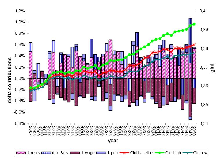
Figure 10 shows a similar decomposition of the dynamics of Gini disposable income disentangling the specific role of different income sources – i.e. labour incomes (d_wage), pensions (d_pen), rents on real estate net of negative interests (d_rents) and interests/dividends on financial wealth – in determining its variation.

Differential contributions to disposable income Gini variation between high and low returns scenarios, 2007–2050.
Source: Authors’ computations on simulated data.
In particular, the figure plots the differential contribution of each income source between the higher and lower returns scenarios (both within a common LC approach). Opposite to wealth inequality, in this case it is worth noticing the crucial role of capital incomes; in fact, the dynamics of the Gini in disposable incomes is positively related to the mean returns on private assets (Table A1).
The key ingredient to explain the underlying logics lies in the cumulated difference between the average net returns on private assets and the general growth of earnings (being zero the real growth of pensions), i.e. r-g. Table 6 shows that this latter cumulated difference ranges from 0.13% according to the lower returns assumptions to 1.28% in the higher returns scenario. Such differential mirrors in an increasing share of capital incomes over time, as reported in Table 7. Since capital incomes are assumed to be a fixed proportion of the underlying stocks (a simplifying hypothesis that can be relaxed) and latter is distributed more unevenly than labour and pension incomes, an increasing share of capital income on overall disposable income implies growing inequality. Thus, with r>g (as it is in the present and likely to be in the next years) wealth coming from the past or received as a gift or bequest is going to be compounded faster than earnings growth (see on this topic Piketty, 2011)
Cumulated contributions to disposable income Gini variation, LC approach, different returns scenarios, 2008–2050 (in percent).
| After_tax pensions | After-tax earnings | Rents on real estate net of liabilities | Interests on financial wealth | d.gini | avg r-g | |
|---|---|---|---|---|---|---|
| 2.low returns | 5.55 | −1.42 | 2.50 | 3.51 | 10.13 | 0.13 |
| 1.Benchmark | 5.28 | −6.69 | 7.57 | 4.92 | 11.08 | 0.61 |
| 3.High returns | 4.79 | −14.70 | 16.89 | 6.89 | 13.88 | 1.28 |
| (3)-(2) | −0.76 | −13.28 | 14.40 | 3.39 | 3.75 | 1.15 |
-
Source: Authors’ computations on simulated data.
Finally, the role of the shares makes also clear the negative contribution to inequality variation of the after-tax earning source despite the future increase in its Gini (not showed here). In fact, the share of labour income on total disposable income is expected to decrease over time, and this fall is stronger the higher the projected returns on wealth due to the increasing relative importance of capital incomes (Table 7).
Cumulated variation in incomes shares (in percent).
| Sources | 2008 | 2050 | 2050–2008 | 2008 | 2050 | 2050–2008 | 2008 | 2050 | (2050)-(2008) |
|---|---|---|---|---|---|---|---|---|---|
| After-tax earnings | 51.0 | 43.8 | −7.2 | 51.4 | 46.2 | −5.2 | 50.7 | 40.0 | −10.7 |
| After-tax pensions | 29.7 | 29.7 | 29.9 | 31.3 | 1.5 | 29.5 | 27.2 | −2.3 | |
| Rents on real estate net of negative interests | 14.6 | 18.3 | 3.7 | 14.1 | 15.1 | 1.1 | 15.2 | 23.7 | 8.6 |
| Interests on financial wealth | 4.7 | 8.2 | 3.4 | 4.7 | 7.4 | 2.7 | 4.7 | 9.1 | 4.4 |
-
Source: Authors’ computations on simulated data.
4. Concluding remarks
The long run distributional effects of demographic transitions and structural reforms in social security, adopted to cope with them, are largely unknown and not easy to predict. In such new scenario, private wealth becomes crucial both in determining overall wellbeing after retirement and, ex ante, in affecting saving/investing as well as retirement decisions. Despite its growing importance, this issue has not yet been analysed in depth, especially in its distributional implications. The present work aims to fill this gap by endowing the Italian dynamic micro simulation model CAPP_DYN with a module accounting for the role of private asset accumulation and spend down. The joint analysis of private wealth accumulation and social security wealth is particularly important in order to get a reliable evaluation of household disposable incomes and standard of living in the coming decades.
Since transitions are likely to affect households’ accumulation patterns, we attempt to account for possible savings reactions by hooking the consumption rule to a life cycle framework. Our main argument points at stressing the relevance of expectations about future resources in current consumption choices in a radical – but very gradual across cohorts – reform scenario. In particular, policy parameters enter into the saving decision by means of subjective expectations about pension outcomes. Since the reform is still in progress and individuals/households seem to adjust slowly their behaviour, the consumption rule we estimate and introduce in the simulation program allows the age structure of the propensity to consume current income to vary along the simulation period according to the internalization process of expectations better than a Keynesian consumption function would do. This semi-structural formulation of consumption equation, coupled with traditional probabilistic approach for other processes and heuristic rules of thumb accounting for stylized facts, allows embodying these tendencies while not neglecting the current empirical evidence and the institutional specificities.
Moreover, we consider the modeling of private wealth transmission among generations as crucial in order to get a more accurate picture of the future distribution of economic resources. To this end, we provide the wealth module with a probabilistic sub-module of intergenerational transfers. We conceive the endogenization of savings and wealth transfers as well as their relationships with inequality as an original contribution of our model to the existing microsimulation literature.
As the behavioural hypothesis adopted can significantly affect results, we compare our semi-structural life-cycle approach with the estimation and the simulation of a non-structural consumption rule, analyzing wealth and disposable income dynamics and their drivers according to the two approaches, especially in a long-term intergenerational perspective.
While a ‘quasi’ life cycle consumption profile, including saving responses to pension reforms, curbs the dynamics of wealth inequality compared to the non-structural approach, results suggest an increasing contribution of intergenerational transfers to the predicted increase in wealth dispersion. Although hypotheses on (the mean of) returns are neutral for the evolution of net wealth inequality, the differential between returns and productivity (r-g) parameters are crucial in affecting the dynamics of disposable income due to cumulated effect on capital incomes shares.
Footnotes
1.
For an updated overview of pension reforms since 1990s, see T-Dymm final report, Section I, Chapter 4 at http://www.tdymm.eu/sites/default/files/Final-Report.pdf.
2.
See Pensim for US and Sesim for Sweden
3.
For a description of the pre-existing structure of CAPP_DYN, see Mazzaferro and Morciano (2008).
4.
The main implication is that feedbacks from wealth to demographic and occupational decision are not allowed for. A further development of the research will be the sequential integration of the wealth module with pre-existing modules.
5.
D’Aurizio et al. (2006) matched the 2002 SHIW wave with anonymous data from a sample survey of customers of the Unicredit group on the assets actually owned. By using advanced econometric techniques, this procedure determines a substantial correction for private bonds and mutual funds, particularly significant for single household and increasing with age. We do not employ the adjusted data in the econometric stage (except for the estimation of the risk propensity), but we replace them in the initial population (2002) in order to simulate more realistic distributions.
6.
CAPP_DYN is a discrete-time annual model, while our main estimation dataset (the Bank of Italy Survey of Household Income and Wealth) has a two-year frequency. This fact causes an underestimation of persistence in the simulated dynamic models. We are aware of this problem, but, at the state of the art a yearly panel data source is not available for Italy. We thus believe the advantages of fitting a better model (especially for the consumption rule) outweigh the drawback of an underestimated persistence in simulation.
7.
In the benchmark scenario, we have adjusted the average return from Muzzicato et al. (2008) – amounting to about 2.5% over the 1970–2007 period – by imputing a lower (very long run) rate of 1.5%. At the same time we adopt a moderate 8% standard deviation, close to that estimated by Cannari, Faiella (2008) for houses prices in Italy.
8.
This aggregate is composed of stocks, mutual funds, private bonds, foreign government bonds, shares of limited liability companies.
9.
Non-risky assets include bank and postal deposits CDs, PCTs, BFPs and government securities. We also added real (tangible) goods other than real estate.
10.
In the benchmark simulation, we assume real returns of 3% with a standard deviation of 18% and an excess of kurtosis of 2.4% for risky assets. These values amount to a weighted average of short, medium and very long run returns for Italy computed by Dimson et al. (2006).
11.
We tested both a time consistent: β = 1 and δ= 0.971→ i = 3%, and a quasi-hyperbolic framework and decided to adopt this latter scenario as a substantial strand of empirical literature supports this attitude in individuals’/households’ saving decisions (see Thaler, 1990). In fact, it provides simulation results more plausible and consistent with stylized facts. Moreover, it softens the impact of a life-cycle framework making the adjustment process in consumption choices slower, in line with empirical evidence. Presentation and discussion of results under the alternative scenario are available upon request.
12.
The last reform by Monti-Fornero (2012), increased significantly mandatory retirement age, further reducing the flexibility which is a typical feature of the NDC systems. As the paper has mainly a methodological content, the version of CAPP_DYN on which the Wealth module has been applied has not been updated to the last pension reforms.
13.
For an analysis of retirement expectations and pension reforms on SHIW, see Bottazzi et al. (2006).
14.
A drop in consumption after retirement still remains to be clarified. Several theoretical and empirical works propose different explanations for this stylized fact (Hurd & Rohwedder, 2008; Laitner and Silverman 2005; Fernandèz-Villaverde and Krueger, 2005. For Italy, Miniaci et al., 2003).
15.
According to SHIW, household head is defined as the person responsible for the household economic management, irrespective of the gender.
16.
Following Ando and Nicoletti Altimari (2004), we divided the household population in five categories: singles, nuclear families (two spouses plus children, if any), non-nuclear families (households with spouses and active children only, not properly composite non-nuclear families), nuclear single headed and non-nuclear single headed.
17.
Financial wealth includes bank accounts, government and corporate bonds, stocks, mutual funds, individual retirement accounts, contractual savings for housing and life insurance policies.
18.
This is a stronger, less realistic assumption. Nevertheless, only few households are selected for receiving an inter vivos transfer more than once or twice in a life cycle so this implicit assumption should be quite innocuous in distributional terms.
19.
On the opposite, the exclusion of such a covariate (which explains much of the selection/outcome equations) in the recipient equation would have implied a much lower variability in the predicted amount of the received transfers compared to the variance in the predicted amount of given transfers. This fact would have ended up making the transfer sub-module work as a progressive tax-benefit module, with obvious distorting rebounds on the transmission of inequality among generations.
20.
It has to reminded that SHIW micro-data overestimate aggregate households’ savings propensity (as these are obtained residually), compared to National Accounts; thus it has been necessary to calibrate initial aggregate savings to these latter values.
21.
This does not prevent in our simulation households to bequeath even generous amounts of wealth as would be, on the opposite, required by a ‘pure’ life-cycle framework.
22.
In the simulation program we do not explicitly account for the role of capital incomes on the household consumption.
23.
In order to avoid the effects of the other components to be affected by the early distribution of wealth and better analyze the accumulation dynamics underlying the wealth module, we proportionally spread the initial wealth of the base population in the first year of simulation on the remaining components.
24.
These components have been calculated in STATA using descogini (Lopez-Feldman, 2006).
Appendix
Table A1 Exogenous parameters (per year).
| Low returns scenario | Benchmark returns scenario | High returns scenario |
|---|---|---|
| Productivity | Productivity | Productivity |
| Same as benchmark | G (average earnings growth) | Same as benchmark |
| “ | 0.88% (2008–2009) | “ |
| “ | 1.00% (2010–2013) | “ |
| “ | 1.20% (2014–2019) | “ |
| “ | 1.90% (2020–2029) | “ |
| “ | 2.00% (2030–2050) | “ |
| Capital gains | Capital gains | Capital gains |
| rh ~N µ=0.75%; sd=8% | rh ~N µ= 1.5%; sd= 8% | rh ~N µ=2.5%; sd=8% |
| rf ~N µ=1.5%; sd=18%; | rf ~N µ=3%; sd=18%; | rf ~N µ=5%; sd=18%; |
| kurt = 2.4% | kurt=2.4% | kurt=2.4% |
| resa=0.9% | resa=0.9% | resa=0.9% |
| Interests and rents | Interests and rents | Interests and rents |
| Same as benchmark | rm ~N µ=3%; sd= 0.5% | Same as benchmark |
| “ | home equity annual rent: 3.5% | “ |
| “ | real interest rate on non-risky AF: 1% | “ |
| “ | real interest rate on risky AF: 3% | “ |
References
-
1
A Micro Simulation Model of Demographic Development and Households’ Economic Behavior in Italy. Discussion paper n. 533Rome: Bank of Italy.
- 2
-
3
Another look at the instrumental variable estimation of error-components modelsJournal of Econometrics 68:29–51.
-
4
The Fourth International Forum of the Collaborating Projects On Ageing IssuesThe Reform of the Italian Pension System, and its Effect on Saving Behaviour, The Fourth International Forum of the Collaborating Projects On Ageing Issues, Tokyo, February, 18th-21th.
-
5
Supplementi al Bollettino Statistico – note metodologiche e informazioni statisticheArchivio storico dell’Indagine sui bilanci delle famiglie italiane, 1977–2004, Supplementi al Bollettino Statistico – note metodologiche e informazioni statistiche, Bank of Italy, Rome.
-
6
Initial conditions and moment restrictions in dynamic panel-data modelsJournal of Econometrics 87:115–143.
-
7
Retirement Expectations, Pension Reforms, and Their Impact on Private Wealth Accumulation. CFS Working Paper Series 2006/10Frankfurt: Centre for Financial Studies.
-
8
House Prices and Housing Wealth in Italy. Discussion Paper n. A4Rome: Bank of Italy.
-
9
L’under-reporting della ricchezza finanziaria nell’indagine sui bilanci delle famiglie. Discussion paper n. 610Rome: Bank of Italy.
-
10
The Worldwide Equity Premium: A Smaller PuzzleEFA 2006 Zurich Meetings, Paper available at SSRN, http://ssrn.com/abstract=891620.
-
11
Consumption over the Life Cycle: Some Facts from Consumer Expenditure Survey Data2004 Meeting Papers 173,.
-
12
The Retirement Consumption Puzzle: Actual Spending Change in Panel Data. NBER Working Papers 13929National Bureau of Economic Research, Inc..
-
13
Health care quality, economic inequality, and precautionary savingHealth Economics 16:327–346.
-
14
Estimating Life—Cycle Parameters from Consumption Behavior at Retirement. Working Papers wp099University of Michigan, Michigan Retirement Research Center.
-
15
Income inequality effects by income source: A new approach and applications to the United StatesReview of Economics and Statistics 67:151–156.
- 16
-
17
The retirement consumption puzzle: a marital bargaining approach. Working Paper 01-04, RANDWashington D.C.: Corporation Publication Department.
- 18
-
19
Department of Economics 0595CAPP_DYN: A Dynamic Microsimulation Model for the Italian Social Security System, Department of Economics 0595, University of Modena and Reggio E., Faculty of Economics “Marco Biagi”.
-
20
Intertemporal Nonseparability or Borrowing Restrictions? A Disaggregate Analysis Using a U.S. Consumption PanelEconometrica 64:1151–83.
-
21
Is There a Retirement Consumption Puzzle in Italy?. IFS Working Paper 03/14London: Institute for Fiscal Studies.
-
22
T-Dymm Final Report - Innovative datasets and models for improving welfare policiesT-Dymm Final Report - Innovative datasets and models for improving welfare policies, http://www.tdymm.eu/sites/default/files/Final-Report.pdf.
-
23
Utility Analysis and the Consumption Function: an Interpretation of the Cross-Section DataIn: K Kurihara, editors. Post-Keynesian Economics. New Brunswick: NJ Rutgers University Press. pp. 388–436.
- 24
-
25
On the Long-Run Evolution of Inheritance: France 1820--2050The Quarterly Journal of Economics 126:1071–1131.
- 26
-
27
Consumption with Habit Formation. CIRANO Working Papers 2000s-39Montreal: Centre Interuniversitaire de Recherche en Analyse des Organisations.
- 28
-
29
Long Run Distributional Impact of Pension Reforms: a Micro Simulation ApproachLong Run Distributional Impact of Pension Reforms: a Micro Simulation Approach, PhD thesis, University of Rome “La Sapienza”.
-
30
Saving, Fungibility, and Mental AccountsJournal of Economic Perspectives, American Economic Association 4:193–205.
-
31
Consumption, habit persistence, imperfect information and the lifetime budget constraint. ECB Working Paper N.251Frankfurt: European Central Bank.
Article and author information
Author details
Acknowledgements
We are grateful to Leandro D’Aurizio, Ivan Faiella, Stefano Iezzi and Andrea Neri for providing us with data adjusted for under-reporting resulting from their work “L’under-reporting della ricchezza finanziaria nell’Indagine sui Bilanci delle Famiglie Italiane”.
We would also like to thank Sergio Nicoletti Altimari for his precious suggestions in the preliminary phase of this work as well as Francesca Gastaldi and Paolo Liberati for their help during the phase of revision.
This work is a synthetic revised version of Simone Tedeschi’s Ph.D thesis. Further details are available upon request.
The opinions expressed here are those of the author and do not reflect the positions of the Bank of Italy.
Publication history
- Version of Record published: August 31, 2013 (version 1)
Copyright
© 2013, Tedeschi et al.
This article is distributed under the terms of the Creative Commons Attribution License, which permits unrestricted use and redistribution provided that the original author and source are credited.