A mate-matching algorithm for continuous-time microsimulation models
- Max Planck Institute for Demographic Research, Germany
Abstract
The timing of partnership formation in closed continuous-time microsimulation models poses difficulties due to the continuous time scale. in this paper the problem is resolved by the concept of a partnership market, which individuals can enter and leave at any point in time over the complete simulation time range. Each individual, who looks for a spouse, remains in the market for a specific period during which searching and matching is performed. To build up synthetic couples, the model imitates a decision making-process. The decision to enter a partnership depends on empirically estimated logit models for the probability that a given woman and a given man will get together, and also on an individual aspiration level regarding a potential partner. A couple is formed if a positive decision has been made and the timing of the partnership formation is consistent with the individual searching periods of the prospective spouses. The algorithm is illustrated by an example in which simulations are run to project a synthetic population, similar to the population of the Netherlands, by using an extended version of the microsimulation tool of the MicMac project.
1. Introduction
To realistically model individual behaviour, the effect of inter-individual interaction has to be addressed. That is, a realistic description of life-course dynamics necessitates the consideration of “linked lives” (Elder et al., 2004; Huinink and Feldhaus, 2009). People cohabit or marry, have children and live in families, and this environment has an impact on their demographic behaviour. it implies that some individual demographic events require that other individuals are linked to a person, and that the relationship between linked individuals may modify their future behaviour, i.e., the behavioural model describing their life courses. For example, in the majority of cases, the decision to have children depends not only on the woman, but also on the potential father and, presumably, additionally on the social network of each (Bernardi, 2003). In a microsimulation, life course events are commonly determined based on empirical distribution functions that rely on data reported for single persons. Individual interaction patterns, like partnership relations and kinship, are often neglected in this context (Ruggles, 1993). This paper investigates one particular problem that arises when including linked lives into a continuous-time microsimulation model: it addresses the onset of partnership (cohabitation or marriage) and the matching of proper mates in continuous time.
As a social science application, microsimulation can be described as an approach that models the dynamics of a system, population, society or economy by modelling the behaviour of its micro-units (typically individuals or single households). The central unit of a demographic microsimulation model is the individual life course, which is characterized by a sequence of demographic events such as birth, marriage, childbirth, divorce, retirement, and death, and the time spans between these events.
In demographic microsimulations, life courses usually evolve along two time scales: individual age and calendar time. A possible third time scale is the time that an individual has already spent in his/her current demographic state, e.g., the time that has elapsed since the individual’s wedding. All time scales can either be discrete (usually in units of years) or continuous (Wolf, 2001; Galler, 1997). In discrete-time models, time advances in discrete steps (commonly in years or months), i.e., the time axis is discretized. At each step, individual attributes and behaviour are updated. In contrast, a continuous-time microsimulation model features a continuous time scale along which events occur, i.e., an event can occur at any instant in time. Generally, for a precise description of population dynamics, continuous-time models are the optimal theoretical choice as a continuous approach most closely mirrors life course development (Willekens, 2009). Furthermore, compared to a discrete-time microsimulation, the processing of a continuoustime microsimulation can be very efficient (Satyabudhi & Onggo, 2008; van Imhoff & Post, 1998). This is because, in a continuous-time microsimulation, individual attributes are only updated when an event occurs. However, continuous-time microsimulations pose some problems when forming relationships that discrete-time models can avoid (van Imhoff & Post, 1998). In discrete-time models, it is convenient to construct mating pools at equidistant time points, e.g., for every year. During simulation, individuals enter these mating pools and undergo mate-matching. In continuous-time models, events occur at exact time points and, in practice, individuals will never experience partnership events at the same time. Therefore, a pool of potential partners cannot as easily be constructed as in discrete time models.
Nevertheless, a common way to establish partnership markets in continuous-time models is to use open mating models. In this class of models, spouses are created as new individuals when needed, rather than selected from already existing members of the population. The main problem of open mating models is their interpretation: it is not realistic to pull an appropriate spouse “out of the hat” when needed. A more realistic way to model mating instead is to use a closed mating model. Here, appropriate spouses are identified from the current members of a population. To ensure that a closed mating model resembles observed mating patterns, it has to be applied to a large enough share of an entire population. Up to now, closed mating models have only been used in the context of discrete-time microsimulation. A reason might be that in continuous-time models the probability that two events will happen at exactly the same time point is zero and thus practically individuals will never experience partnership events at the same time. As a consequence, in a continuous-time model, a pool of potential partners is hard to identify.
In this paper it is proposed to determine a pool of potential partners by establishing a partnership market which individuals can enter and leave at any point in time during the simulation. As soon as an individual starts to look for a spouse, he/she becomes part of the market and stays there until mate-matching is finished. To match individuals, an algorithm is needed to determine appropriate partners: Who should be linked to whom? Humans mate assortatively (Blossfeld & Timm, 2003; Kalmijn, 1998); that is, partners are not chosen randomly but are selected according to preferences. Typically, spouses are similar with respect to certain attributes, and synthetic couples should reflect this habit. Accordingly, a two-fold approach is suggested to build up synthetic couples: First, to each individual a random value is assigned that captures his/her aspiration level regarding a partner. An empirical likelihood equation reveals the probability that a given woman and a given man form a couple. Subsequently, a decision-making process is simulated as to whether two individuals mate, applying individuals' aspiration levels and their matching probability.
The rest of the paper is structured as follows. Section 2 is a brief review of mate-matching algorithms already proposed for microsimulations. Here special focus is put on ideas and techniques that are useful for conducting mate-matching in continuous-time models. Section 3 describes a novel mate-matching procedure for continuous-time microsimulation and a critical evaluation of its capabilities. The approach is illustrated by running a microsimulation for a synthetic population reflecting characteristics of the Netherlands population. Results are given in Section 4. The paper concludes by validating the new procedure and by providing an outlook to future work.
2. Review of mating models for microsimulation
Commonly, in microsimulation models two approaches are used to match individuals for partnerships: open mating models and closed mating models. In open models, appropriate spouses are created anew, when needed, while in closed models, partners are identified among already existing individuals. As the interpretation of an open model is difficult, here a decision is made for the usage of a closed mating model.
In a closed model, partners for marriage and consensual union have to be found among existing individuals. Besides the time when couples are formed, the following issues have to be addressed:
How can one determine which individuals are in the (mating) pool or pool of eligible partners?
Who matches whom?
What are the mating rules?
All previous closed mating models were realized in discrete-time microsimulation models, so this review is restricted to discrete-time models. The idea is to inspect existing closed mating models to whether they can be adopted to also work in continuous time. In discrete-time models, assigning individuals to a mating pool proceeds generally as follows: In a discrete-time microsimulation model, time changes in discrete steps. After each step, all individuals of the model population are inspected as to whether they will experience an event during the next interval and, if so, which event this will be. In case an individual is scheduled to experience the onset of a partnership, he/she is marked as searching for a spouse. At each time step, after every member of the population has been inspected, all searching individuals are collected in a partnership market. That is, “a partnership market” is a construct used to pool all those individuals who are looking for a spouse. As a partnership market allows collecting all eligible partners, its construction in any case is deemed useful also in a continuous-time setting.
Generally, to build synthetic couples of the individuals pooled in the partnership market, two main problems have to be solved: Who mates whom? and what data are needed to construct couples that resemble actual/observed ones? Both questions concern the mating rules that are applied to match individuals. Generally, two types of mating rules can be found in microsimulation models: stable and stochastic (Perese, 2002). Stable mating rules aim at producing a set of stable matings (see also the “stable marriage problem” in Gale and Shapley (1962)). Stochastic mating rules use stochastic experiments to decide on the success of potential pairings. All mating rules make use of a compatibility measure to determine the quality of a match. The pros and cons of stable mating rules have been discussed extensively by Bouffard et al. (2001) and Leblanc et al. (2009); in summary, they find that stable mating rules produce too many “extreme” pairings, such as couples with extreme age differences. Stochastic mating rules are an option to overcome this problem.
This review is restricted to stochastic mating rules. First compatibility measures are discussed, and then stochastic mating rules are described.
2.1 Compatibility measure
A compatibility measure transforms female and male attributes into a numeric index which quantifies how compatible a woman and a man are. Commonly, values between zero and one are used to express compatibility, with a large value indicating high compatibility. Likewise, a small value points to incompatibility.
Some notation:
At some point in time the partnership market comprises m women and n men
The female attributes are denoted by wi, i = 1, …, m, and the male attributes by mj, j = 1, …, n,. Typically, such attributes can be represented by a vector, and the different components of wi and mj, respectively, quantify characteristics such as age, educational attainment, etc.
The set F comprises all wi and the set M all mj.
The compatibility measure C is defined as the following mapping
If C(wi, mj) > C(wk, mj) for two females i and k and the same male j, then the pairing of i and j shows a better agreement than the pairing of k and j. Commonly, the elements of wi and mj only give age and educational attainment of males and females. Bacon and Pennec (2007) provide an extensive review of attributes employed in mating models.
Two different specifications of C are typically used: distance functions and the likelihood of a union between potential pairings. Distance functions measure the discrepancy in the attributes of spouses; for example the following exponential distance function (Perese, 2002):
where ai and ei indicate the age and the educational level of a woman i, and aj and ej the respective values of a man j. Using distance functions to measure compatibilities is not unproblematic. The main problem is that distance functions quantify the quality of a pairing in a very simplistic way, for example, not considering possible effects of individual attributes measured as a nominal scale, like race. A more realistic way to determine the quality of a pairing is to use the empirical likelihood of a pairing.
The likelihood of a union between potential pairs can be quantified by logit models (Perese, 2002; Bouffard et al., 2001). The model predicts the probability that two individuals, each with given attributes, form a partnership. Data on observed couples are used to estimate the coefficients of these models. According to the theory of assortative mating, partners tend to have similar ages and similar levels of education (Kalmijn, 1998). Therefore, ideally, the estimated coefficients are in accordance with the theory of assortative mating (Bouffard et al., 2001; Leblanc et al., 2009). In order to account for different types of partnerships (cohabitations and marriages) and to differentiate between first and higher order partnerships, typically more than one logit model is applied.
2.2 Stochastic mating rules
In a stochastic mating model, the compatibility measure between a woman and a man determines the probability of a respective match, and the outcome of a stochastic experiment determines whether a match between two potential spouses occurs. A stochastic matching procedure ensures that individuals with a low compatibility also have a chance to get matched. With regard to their compatibility, constructed couples are thus not necessarily optimal ones. As a result, the occurrence of “extreme” matchings is less likely, which is a big advantage over stable mating rules.
In microsimulation models, basically, three variants of stochastic mating are applied, depending on whether and which sex dominates the choice of spouses (male-, female- or mixed-dominant algorithms). In male-dominant mate-matching algorithms, men choose their spouses from a list of eligible women (of fixed or random length) in accordance with their compatibility (see e.g., Perese (2002)). In a female-dominant mate-matching algorithm, the roles of women and men are simply reversed: Women choose from a list of potential spouses (see e.g., Hammel et al. (1976, ch. 9) and Kelly (2003)). In a mixed-dominant mate-matching procedure, both sexes are treated equally. Here two variants can be distinguished: In the first variant, from the partnership market an individual is randomly selected to look for a spouse. This individual then randomly chooses his/her actual spouse from the opposite-sex candidates with the highest compatibility (Wachter, 1995). In contrast, in the second variant, initially the compatibility measure between all potential pairings is determined, and then couples are constructed. The latter variant goes back to the work of Vink and Easther (Bouffard et al., 2001).
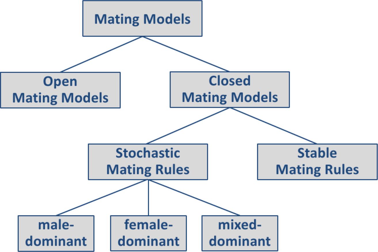
Figure 1 shows the presented classification of mating models and mate-matching algorithms designed for microsimulation models.
In conclusion, the following findings can be summarized:
Closed models are easier to interpret than open models, and they enable us to study the effects of mating processes on the population composition.
The construction of a partnership market allows us to collect all eligible partners.
To measure the compatibility between two persons, computing the likelihood of a potential pairing is more appropriate than using a distance function.
Stochastic mate-matching procedures resemble actual data better than stable mating procedures, but the outcome of a stochastic mate-matching algorithm is not significantly affected by the chosen variant (male-, female-, or mixed-dominant).
Accordingly, the present mate-matching algorithm uses a closed model that embodies a mixed-dominant, stochastic, mate-matching procedure. The details of the approach are described in Section 3.

Classification of mating models and mate-matching algorithms for microsimulation.
3. A mutual mate-matching procedure in continuous time
In continuous-time models the probability that two events will happen at exactly the same time point is zero and, in practice, individuals will never experience partnership events at the same time. Due to this design, a pool of potential partners is hard to identify. A way to approach this problem is to include in the mate-matching algorithm the scheduling of events and the construction of a partnership market that individuals can enter or leave over the complete simulation time range. The processing of the present mate-matching procedure can be summarized as follows:
individuals enter the partnership market,
potential couples are built and tested for conformance,
if a potential couple is compatible concerning its partnership formation time and concerning its characteristics it is realized.
The whole approach is now described at length, considering cohabitation and marriage as two separate types of partnership.
3.1 Entering the partnership market
In a continuous-time microsimulation, empirical waiting times (derivable from empirical rates) determine the occurrence and timing of events. That is, life courses can be constructed as sequences of waiting times to next events (Gampe & Zinn, 2007). As a direct consequence, partnership formation times are already known in advance. This knowledge is used when constructing a partnership market for a continuous-time microsimulation: an individual is determined to enter the partnership market at the moment when the waiting time to a partnership formation event starts. That is, as soon as a marriage or cohabitation event has been simulated, an individual joins this market. To be able to explain this circumstance better, consider the following example: Simulation starts at time ts when a woman is a0 years old. She has never been married and is childless at this time. Conditional on her current state, her age, and the current calendar time, a waiting time of w = 3.6 years to a marriage event is simulated. The woman enters the market at time ts and her waiting time to marriage is w = 3.6 years.
3.2 Scheduling of partnership events
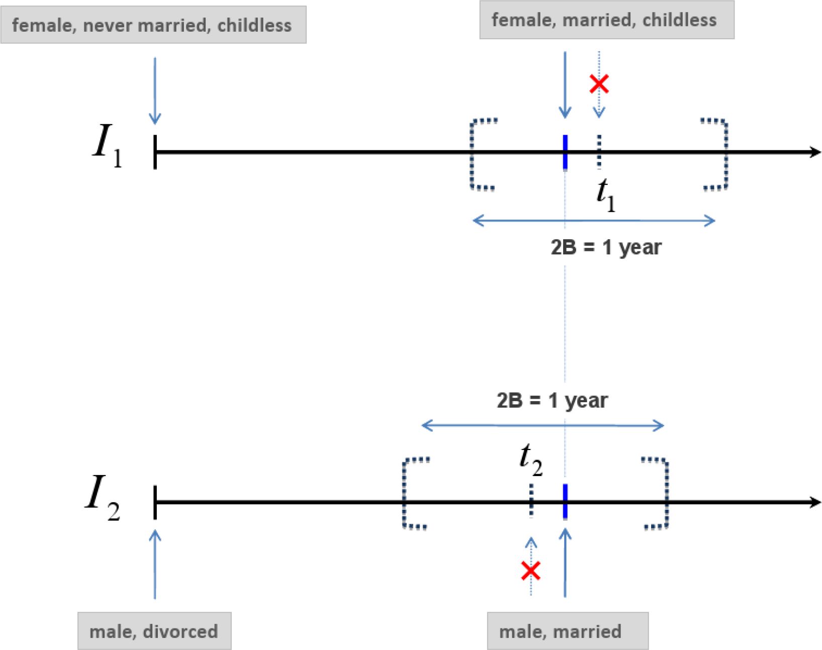
A partnership (marriage or cohabitation) has to have a clearly defined formation time, i.e., a joint mating time of two spouses. However, as already mentioned, in a continuous-time model the probability of a concurrent event is zero. As a consequence, two individuals will never have identical mating times. An option to nevertheless conduct mate-matching is to slightly adjust mating times computed by the microsimulation model to obtain joint mating times. An example helps illustrating the respective procedure: A woman I1 experiences the onset of a partnership at time t1, and a man at I2 time t2. Without loss of generality, it is assumed t2 < t1. One way to compute a formation time of a partnership between I1 and I2 is , c ∈ [0,1]. Then, instead of t1 and t2, for both I1 and I2 the adjusted is used as starting time of a partnership. The new partnership formation time is located between t1 and t2. Whether is closer to t1 or to t2 is determined by the parameter c. A setting of c = 0.5 results in the mean of t1 and t2. Changing simulated event times this way means changing the outcome of the microsimulation model. For example, if it is assumed that for I1 a marriage event has been simulated to happen at January 10, 2014 (t1) and for I2 a marriage event has been simulated to happen at January 1, 2012 (t2), then with c = 0.5 their new joint partnership formation time () would be January 4, 2013. Using January 4, 2013, however, as wedding date means shifting the originally simulated wedding times for more than one year.

Woman I1 experiences a marriage event at time t1. Man I2 experiences a marriage event at time t2. As t1 ∈ [t2 − 0.5 years, t2 + 0.5 years] and t2 ∈ [t1 − 0.5 years, t1 + 0.5 years] both individuals have overlapping searching periods and might meet during the mating process.
Hence, they can be considered as potential spouses. Their formation time would be if they were actually linked in the mate-matching algorithm.
Therefore, to avoid significant change and bias to the outcome of the microsimulation model, it has to be assured that t1 − t2 is small. Accordingly, I1 and I2 can only be regarded as potential spouses if their simulated times t1 and t2 are close enough. Here, t1 and t2 are defined as close enough, if t1 ∈ ┌2 and t2 ∈ ┌1, where
┌1 = [min(ts,u1,t1 − B), max(t1 + B,tE)] and
┌2 = [min(ts,u2,t2 − B), max(t2 + B,tE)].
tS is the simulation start time, tE the simulation stop time, and ui is the time of the event that Ii has experienced previous to the upcoming partnership formation event, i = 1,2. B is an arbitrary time period, but which is commonly shorter than one year. ┌i is called the “searching period” of Ii.2 ┌i starts soonest with Ii’s entry into the partnership market. For consistency, at the earliest, the searching period starts at simulation start time and, at the latest, ends at simulation end time.
With respect to this definition, only individuals can meet if their searching periods overlap. Subsequently, it is B = 0.5 years and c = 0.5. The latter results in . Figure 2 illustrates the adjustment of event times using an example. Section 4.2 deals with how shifting events in the suggested way changes the output of the stochastic microsimulation model.
3.3 Compatibility and individual characteristics
Even if the searching periods of mating willing individuals overlap, their characteristics might not match. Therefore, besides event times, individual characteristics also have to be checked for conformance. For this purpose, a compatibility measure is used such as introduced in Section 2.1. As distance functions measure the quality of pairings very simplistically, logit models are employed to evaluate how well the characteristics of potential spouses agree. Which covariates will enter the logit models depends on the state space of the actual application. In this paper a generic microsimulation model is assumed; i.e., the state space is not fixed. Only individual age and sex are mandatory attributes. Depending on the problem to be studied, different relevant demographic states will be considered. Obviously, only those covariates can be included in the logit models that are in the state space. If, for example, educational attainment, children ever born, or ethnicity are included in the state space, these attributes are natural candidates for covariates in the logit models. For a pair of individuals, the compatibility measure gives, conditioned on the considered attributes, the probability of a union.
3.4 Mate-matching procedure
The partnership market is implemented using a so-called marriage queue M. The marriage queue consists of all unpaired individuals who are looking for a partner (because of a simulated partnership event). Each individual in the queue is equipped with a stamp that indicates the time of the upcoming partnership event.
When determining how many potential partners an individual can meet, individuals have constraints on the social network size they can perceive. Humans are thought to be limited to social networks with approximately 150 members (Hill & Dunbar, 2003). Considering this fact, for each individual the maximal number of potential spouses is restricted. An upper bound is set that follows a normal distribution with expectation μ = 120 and standard deviation σ = 30.
Furthermore, to each individual a random value is assigned that captures his/her aspiration level regarding a partner. This aspiration level takes values between 0 and 1. If the compatibility measure between an individual and a potential spouse exceeds the aspiration level, he/she accepts the pairing. Thus mate-seekers are satisficing (Simon, 1990): different candidates are inspected until one is found that “meets the expectation". In the proposed algorithm, individuals reduce their aspiration level by δA,δA ∈ [0,1], every time they are involved in an unsuccessful encounter. This way their chance to find a mate the next time is increased. The reduction of the aspiration level with each rejection corresponds to a strategy proposed by Billari (2000) and Todd et al. (2005). They suggest using individual aspiration-based heuristics to model human mate-choice processes. The basic idea is that if the traits of a potential spouse meet or exceed an individual’s aspiration level, a partnership is formed. Aspiration levels are adjusted according to offers and rejections received by others. Here this approach is adapted by reducing the aspiration levels of individuals who date but reject each other.
The individual aspiration levels are assumed to follow a beta distribution. Based on the theory of initial parental investment, women are assumed to be “choosier” than men concerning their partners (Trivers, 1972; Buss, 2006). However, the degree of “choosiness” of females and males varies with age. Women tend to decrease their requirements with declining fecundity. When they are in their early thirties, they are less demanding than at younger ages. For single women older than 35, the “ticking of the biological clock” even leads to a considerably increased effort to date men (Pawlowskia & Dunbar, 1999). While after age 40, women tend to be more “choosy” again (French & Kus, 2008). Although socio-economic factors play a role in this context, too, only the age trajectory is considered here. Men, however, behave differently. When they are young, men are more involved in short-term relationships, and therefore are more interested in the number of sexual partners, not so much in the quality of a relationship (Buss, 2006). As a consequence, they are less selective concerning the traits of a partner. However, when men start to look for long-term relationships, willing to establish a family and to invest in offspring, their behavior changes, and their level of “choosiness” increases. In this approach, 30 is selected as the age when men start to intensively look for a long-term spouse. To account for the variability in the degree of aspiration, the beta distribution is parameterized accordingly. The parameter values of the beta-distribution are gender-specific and vary with age (see Figure 3).
Parameters and suggested parameter values for the present stochastic mate-matching procedure.
| Description | Parameter | Value |
|---|---|---|
| Intersection of searching periods | B | 0.5 |
| Upper bound of number of potential spouses | N | normally distributed, μ = 120, σ = 30 |
| Individual aspiration level | ai | beta distributed, gender- & age-dependent (cp. Figure 3) |
| Decrement of aspiration level in case of rejection | δA | 0.1 |
| Bound for small pool size | sp | 10 |
| Decrement of aspiration level in case of small pool size | δB | 0.3 |
An important aspect is the size of the pool of potential spouses. If it is small, it is not reasonable to assume a very selective seeker. To increase the chance that each individual finds a partner, it is assumed that, if a seeker faces less than sp potential partners, he/she reduces the aspiration level by δB,δB ∈ [0,1] additionally to the reduction δA induced by having been rejected.
All parameter values for the mate-matching procedure are given in Table 1. For Western Europe, the chosen parameterization is reasonable as the result of the case study in Section 4.2 will illustrate. Furthermore, a small sensitivity analysis in Section 4.2 supports the feasibility of the chosen parameterization.
To actually construct synthetic couples, a modified version of the first variant of the mixed-dominant mate-matching procedure that was introduced in Section 2.2 is used. If for an individual Ii an upcoming partnership event has been simulated, i.e., Ii enters the searching phase, the following steps are performed:
The searching period ┌i of Ii is determined, and his/her level of aspiration ai is generated.
If the marriage queue M is empty (i.e., the partnership market is empty), Ii is inserted into M.
Otherwise
a random number N is drawn, normally distributed with expectation μ and standard deviation σ, to define the size of the social network of Ii. If N is greater than the current number NM of individuals in the marriage queue, N = NM is assigned.
Randomly, out of M, N individuals are taken whose searching periods overlap ┌i, and they are inserted into the so-called working marriage queue W.
Individuals of the same sex as Ii and individuals who do not meet some minimal criteria are removed from W.
If W turns out be empty, Ii is inserted into M.
Otherwise (if W is not empty) the following procedure is triggered:
If W contains less than sp individuals, we reduce the aspiration level of Ii to ai = max(0, ai − δB), and
j = 1 is initialized.
The jth individual Ij is taken of W. The aspiration level of Ij is denoted by aj. The compatibility measure cij = C(wi, mj), or cij = C(wj, mi), respectively, between Ii and Ij is computed. If ai < cij and aj < cij, the individuals Ii and Ij get paired, and Ij is removed from M.
Otherwise, the aspiration level of Ii is reduced to ai = max(0,aj − δA), the aspiration level of Ij to aj = max(0,aj − δA), and j is incremented by 1.
Steps (iii) and (iv) are repeated until either is paired or all individuals of W have been inspected.
If no appropriate spouse can be found for Ii, he/she is enqueued into M.
In other words, if Ii fails to find an appropriate spouse at the first try, he/she joins the marriage queue. Here Ii stays until a new individual enters the market, encounters Ii, and both agree to mate.
The terms “marriage queue” and “working marriage queue” as used in the description were introduced by Hammel et al. (1990). To select individuals from the working marriage queue, the following minimal criteria are used: no incest, no remarriage of previously divorced couples, and no extreme age differences between the spouses.
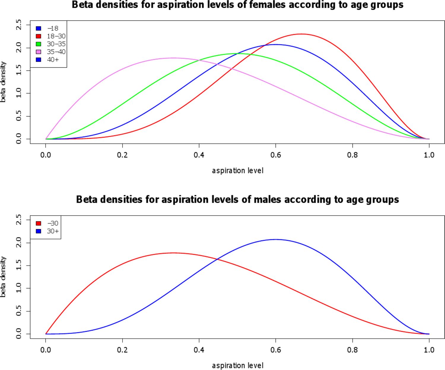
Densities of the beta distributions that are used to determine aspiration levels regarding partners. The densities vary with gender and age. For females, four different curves are applied: one below age 18, one for ages between 18 and 30, one between ages 30 and 35, and one after age 40. For males, two different curves are applied: one for males younger than 30 and the other after age 30.
3.5 The difficulty of getting everybody matched
In a continuous-time microsimulation, events and waiting times to events are simulated based on empirical rates. Therefore, the computation of the entry of an individual into the searching and mating phase relies on observed behavior. The mate-matching procedure proposed here mimics human mating as a decision process. That is, matches that are created during simulation are the outcome of intended behavior. Consequently, not all individuals who engage a mate search phase during simulation will find a partner. Reasons for this are competition with others or simply a short supply of spouses with compatible characteristics. In other words, the presented mate-matching algorithm does not guarantee that each searching individual (i.e., each individual who is part of the partnership market and therefore an element of the marriage queue) will be paired. Mate-matching fails if an individual is not able to find within his/her searching period a spouse with compatible characteristics. In order to be successful, each seeker has to have access to a rich enough pool of potential spouses. This can only be assured if the model population maps a large proportion of an actual population.
Notwithstanding, if the searching period of a “mating-minded” individual (who should find a partner but did not succeed) expires, three options exist:
Extend the searching period. The individual remains in the partnership market, i.e., in the marriage queue.
Return the individual to the model population unpaired. The individual is removed from the marriage queue. He/she is again available to experience a partnership event.
Let an appropriate spouse immigrate or the individual emigrate. The individual is removed from the marriage queue.
The last idea is borrowed from open models, where an appropriate spouse may be created “ex nihilo”.
Each of these three options entails a major difficulty. Extending the searching period (option A) means shifting the time of the partnership event (onset of marriage or cohabitation). Rejecting a seeker (option B) implies ignoring an already scheduled event. Allowing too many emigrating mate seekers or too many immigrating spouses (option C) spoils the representativeness of the model population. Consequently, in order to assure plausible outcomes, searching periods that expire without success should be an exception.
4. Mate-matching in practise
To illustrate the developed algorithm it was included into the MicMac microsimulation tool (Zinn et al., 2009; MicMac project, 2011). Simulations were run to project a synthetic population which resembles the population of the Netherlands. The state space employed for this purpose consisted of the following elements (variables with corresponding values given after the colons, separated by semi-colons):
gender: female; male
marital status and living arrangement: living at parental home and never married; married for the first time, but never lived in a union before; married for the first time and cohabiting before; remarried; living alone and never lived in a union before; living alone but cohabiting before; living alone and married before; first cohabitation; higher order cohabitation but never married before; cohabitation and married before
fertility: childless; one child; two children; three or more children
educational attainment: low (primary education only); medium (lower secondary school); high (upper secondary or tertiary education)
mortality: dead; alive
Simulations were run over 17 years, starting on January 1, 2004 up to December 31, 2020. During simulation, the focus was set on individuals aged between 0 and 63. The initial population consisted of 139,048 males and 134,910 females (which corresponded to 2% of the actual Netherlands population aged 0 to 63 on January 1, 2004). During simulation, individuals could experience the following events: giving birth (for females), leaving parental home, launching a cohabitation, marrying, getting divorced or separated, change their educational level, and death.
To assure that each “mating-minded” individual was matched, option A of Section 3.5 was applied: if an individual was not successful during his/her searching period, the timing of his/her partnership onset was shifted.
4.1 Data
The initial population and transition rates are the essential parameters of any microsimulation. For the example, they were estimated using different European data sources. The EUROPOP 2004 projections for the Netherlands (baseline scenario) provided by EuroStat3 were used. This data set comprises (projected) information on mortality and fertility in the Netherlands for the years 2004 to 2050. Further the Fertility and Family Survey for the Netherlands conducted between February and May 2003 was used. This survey contains micro-information on fertility behavior and changes in marital status. Data on educational attainment were taken from Goujon (2008).
The initial population was constructed using the method of iterative proportional fitting (Kruithof, 1937; Deming & Stephan, 1940). To estimate fertility rates and transition rates regarding marital status, a slightly modified version of MAPLE (Impicciatore & Billari, 2007) was employed. (The initial population and transition rates are available on request from the author.)
The proposed mate-matching procedure requires the computation of compatibility measures between potential spouses. For this purpose, four logit models (see Section 2.1) were used. Each model describes the probability to enter a specific partnership type from the perspective of the male spouse:
Model 1: entering first cohabitation;
Model 2: entering higher order cohabitations;
Model 3: entering first marriage;
Model 4: entering higher order marriages.
An individual who marries his/her common-law spouse already chose him/her when entering the cohabitation. Therefore, in the two latter models, only such marriage events are considered which are not preceded by cohabitations. For estimating the models, the first wave of the Netherlands Kinship Panel Study (NKPS) was used (Dykstra et al., 2005). Only partnerships that started in the years from 1990 to 2002 were included. A data set was constructed that contains for each observed couple a record consisting of
the age of the male spouse,
the age difference between the female and the male spouse (in integer years),
the levels of educational attainment for each spouse,
an indicator whether the female spouse was married before, and
the number of children that the spouses have with former partners.
This sample design is retrospective, i.e., in the data the attributes of female and male spouses were sampled conditional on being paired. To accurately estimate a retrospective regression model, case and control sampling fractions have to be consisted. However, in the present setting such data were not available because it cannot be observed who in reality did not mate. To add information about controls nonetheless, for each observed couple a synthetic couple was built by randomly assigning to each male spouse a female who was not his observed partner. The response variable was set to one in the case a couple had been observed. Otherwise, the response variable was set to zero. Unfortunately, conducting mate-matching requires a prospective design: to measure the compatibility of a pairing, the likelihood that two individuals with certain attributes mate is needed. A mandatory condition of a prospective model is that case and control fractions are made up by the source population, i.e., the sampling has to be random. In this mate-matching procedure, compatibility between two potential spouses is measured on a relative scale, depending only on the attributes of two individuals, and not on the composition of the pool of available candidates. Therefore, for present purposes the estimation of a prospective logit model is suitable (see also Prentice and Pyke (1979)).
Regression results of Model 1 (entering first cohabitation) and 2 (entering higher order cohabitation).
| Model 1 | ||
|---|---|---|
| Variable | Coefficient | p-value |
| Age of male | 0.0521 | 0.0046 |
| Age difference (age of male – age of female) | ||
| greater than 9 | −2.9876 | <0.001 |
| from 7 to 9 | −1.4633 | <0.001 |
| from 4 to 6 | −0.4862 | 0.0108 |
| from −3 to 3 | 0 | |
| from −6 to −4 | −1.4360 | <0.001 |
| from −10 to −7 | −2.8137 | <0.001 |
| smaller than −10 | −3.0582 | <0.001 |
| Difference in educational level | ||
| male is higher or equally educated | 0.6424 | <0.001 |
| Marriage history of female | ||
| female was married before | -0.2811 | 0.1833 |
| Number of potential pairs: 1078 | ||
| Model 2 | ||
|---|---|---|
| Variable | Coefficient | p-value |
| Age of male | 0.0550 | 0.0013 |
| Age difference (age of male – age of female) | ||
| greater than 10 | −3.5428 | <0.001 |
| from 4 to 10 | −3.5428 | <0.001 |
| from −3 to 3 | 0 | |
| from −10 to −4 | −1.0105 | 0.0021 |
| smaller than −10 | −3.1277 | 0.0196 |
| Difference in educational level | ||
| male is higher or equally educated | 0.7825 | 0.0148 |
| Children with former partner | ||
| female has children | 1.6754 | <0.001 |
| Number of potential pairs: 394 | ||
4.2 Results
4.2.1 Evidence from the compatibility measure
The coefficients of the estimated logit models are summarized in Tables 2 and 3. In all models, a positive effect can be observed if the male was higher/equally educated than/as the female. Generally, no significant effect of the marriage history on the mating propensity of the male can be detected. However, the results indicate that, when they married or cohabitated for the first time, men were more prone to mate women who had not been married before. Women and men who mated were more likely to be of the same age. The effect is stronger in the case of firstorder marriages and cohabitations. In all four models, the direct effect of the age of the male is very small. Modeling compatibility by partnership order might be a reason for this phenomenon. First partnerships are usually started at younger ages, while higher order partnerships follow later in life. Therefore, a man’s age at partnership onset is already indirectly described by the partnership type. In the analysis, men had a higher probability to undergo a higher order cohabitation with a female who had already had children with former partners. Surprisingly, for the other partnership types, no significant effects of the presence of children with former partners on a male’s mating probability could be observed.
Regression results of Model 3 (entering first marriage) and 4 (entering higher order marriage).
| Model 3 | ||||
|---|---|---|---|---|
| Variable | Coefficient | p-value | ||
| Age of male | 0.0646 | 0.0650 | ||
| Age difference (age of male – age of female) | ||||
| greater than 10 | −3.3997 | < 0.001 | ||
| from 7 to 10 | −1.4934 | 0.0110 | ||
| from 3 to 6 | −0.8026 | 0.0692 | ||
| from −2 to 2 | 0 | |||
| from −5 to −3 | −1.5026 | 0.0263 | ||
| smaller than −5 | −4.3357 | < 0.001 | ||
| Difference in educational level | ||||
| male is higher or equally educated | 0.8493 | 0.0525 | ||
| Marriage history of female | ||||
| female was married before | −0.4314 | 0.4873 | ||
| Number of potential pairs: 198 | ||||
| Model 4 | ||
|---|---|---|
| Variable | Coefficient | p-value |
| Age of male | −0.0120 | 0.6618 |
| Age difference (age of male – age of female) | ||
| greater than 8 | −2.9174 | < 0.001 |
| from 4 to 8 | −1.6287 | 0.0547 |
| from −3 to 3 | 0 | |
| smaller than −4 | −3.2270 | < 0.001 |
| Difference in educational level | ||
| male is higher or equally educated | 1.2949 | 0.0743 |
| Number of potential pairs: 82 | ||
4.2.2 Re-estimating empirical transition rates
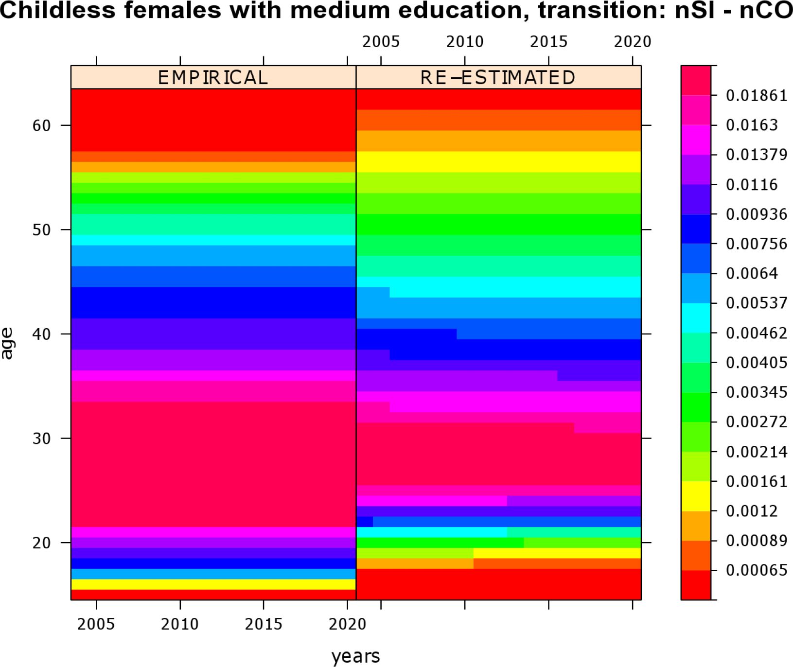
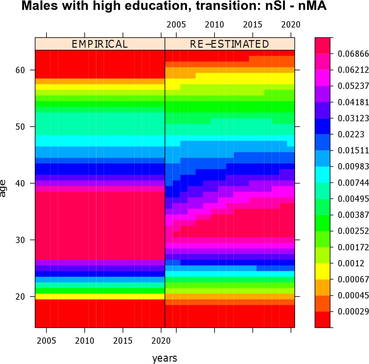
To assess the quality of the proposed mate-matching strategy, validating the simulation output is a good and useful practice. Besides basic validation of the simulation output, important hints for model improvement can be gained from careful analysis of the results. During the mate-matching process several simplifying assumptions were made, e.g., shifting event times, and these may have an undue impact. A very basic validation step is the re-estimation of the empirical transition rates which were used as input, by occurrence-exposure rates (Keiding, 1990). To smooth these rates, a two-dimensional P-splines technique was employed (Currie et al., 2006) that has been implemented in an R package named MortalitySmooth (Camarda, 2009). The re-estimation of rates shows that a simulation with mate-matching causes consistent output. Some results are plotted in Figures 4 and 5. Both figures are level plots4. Empirical rates along with reestimated rates are presented. Rates are given along calendar time and age. Their values are depicted on a “rainbow” color scale: red areas correspond to very low rates and violet-pink areas correspond to high rates. Figure 4 shows transition rates of childless women with a lower secondary (medium) education who experience a transition from “being single after leaving parental home” to “first cohabitation”. Figure 5 depicts transition rates of highly educated males who experience a transition from “being single after leaving parental home” to “first marriage". During simulation both sets of transition rates varied along age but were held constant over calendar time. Figure 4 reveals that, for women with a lower secondary education, empirical and reestimated marriage rates are almost identical, i.e., here the proposed mate-matching procedure does not significantly change the output of the simulation model.
Figure 5 shows that, for highly educated men, the proposed mate-matching procedure causes a slight postponement of partnership onsets in the first simulation period. Especially at higher ages, re-estimated marriage rates are slightly lower than the empirical ones. However, considering the precision of the used rates scale, the observed differences are very small. In summary, the results obtained mean that the re-estimation of the transition rates confirms the general suitability of the proposed mate-matching procedure.

Re-estimation of transition rates of childless females with a lower secondary (medium) education who experience a transition from “being single after leaving parental home” (nSl) to “first cohabitation” (nCO).

Re-estimation of transition rates of highly educated males who experience a transition from “being single after leaving parental home” (nSI) to “married” (nMA).

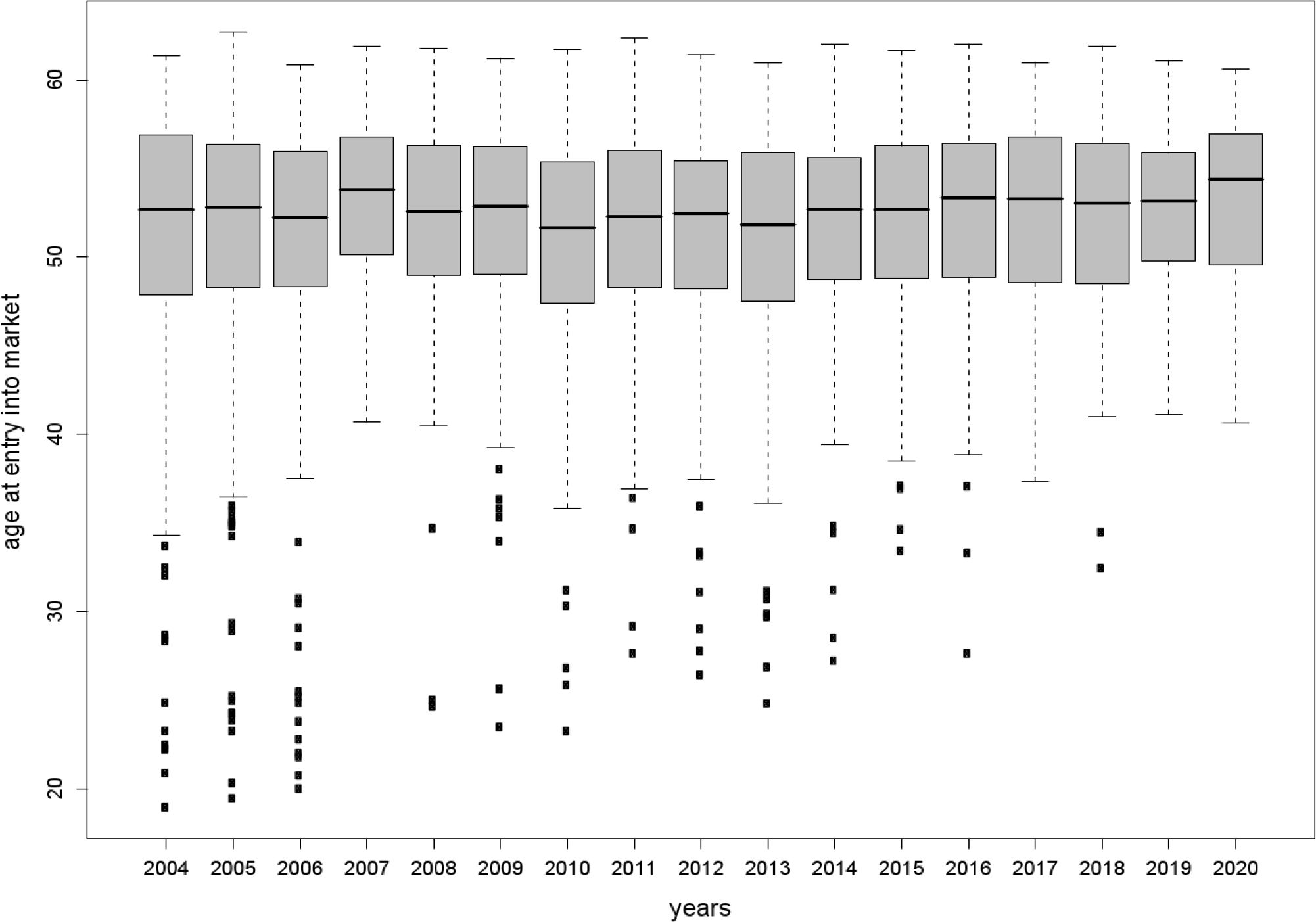
Age distribution of unsuccessful seekers at the time when they enter the partnership market.
4.2.3 Analyzing the pool of unsuccessful seekers
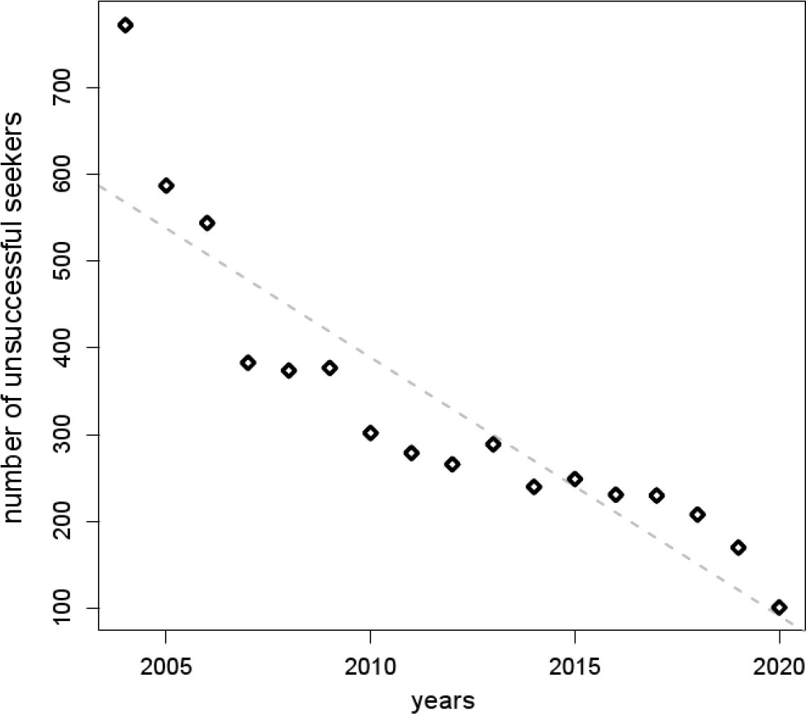
Analyzing the simulated partnership market over time is a way to reveal whether its dynamics resembles human mating behavior. In particular, the composition and the development of the pool of unsuccessful seekers is of interest. During the simulation, 40,585 partnership formations were performed, 19,050 due to marriage and 21,535 due to cohabitation. Thus, 8,170 individuals successfully entered and left the partnership market. Because the algorithm could not find a proper spouse in time, the searching period of approximately ten percent of all seekers had to be extended. Over 17 years of simulation, 5,397 individuals had entered the market without finding a spouse. Figure 6 displays the age distribution of unsuccessful seekers according to the year when they had entered the partnership market. Individuals who initialized a partner search at older ages remained more often unpaired than their younger counterparts. This phenomenon occurred because during simulation the synthetic mating pool for individuals at older ages was not as rich as it was for younger persons. Consequently, for older individuals the chance of finding an appropriate spouse was relatively small. Figure 6 also shows that the age distribution of unsuccessful seekers did not significantly change over the simulation horizon. These findings were contrasted with the number of unsuccessful seekers along the year (see Figure 7). A decline along calendar time is obvious. In summary, along calendar time the number of unsuccessful seekers decreased, but the age distribution of unsuccessful seekers remained stable. This phenomenon is caused by the age structure of the model population. Generally, at older ages only a small proportion of individuals enters the partnership market. As the model population ages during simulation, over time the number of mature adults who enter the market however goes up. Therefore, for them the chance of finding an assortative mate increases, and in the synthetic pool the number of aged individuals who remain unpaired shrinks. But still, compared to younger seekers, the mating pool of older adults is reduced, e.g., due to mortality or a high proportion of married persons at the same age. Decreasing the aspiration level of elderly people is an option to increase their chance to find a partner. However, this also means to allow constructing non-assortative matches, and thus building couples whose attributes do not resemble the attributes of observed couples – a property a mate-matching procedure should guarantee. That is, decreasing the aspiration level of elderly people impairs the proposed mate-matching strategy rather than to improve it.

Number of unsuccessful seekers according to the year when they initialize a partner search.
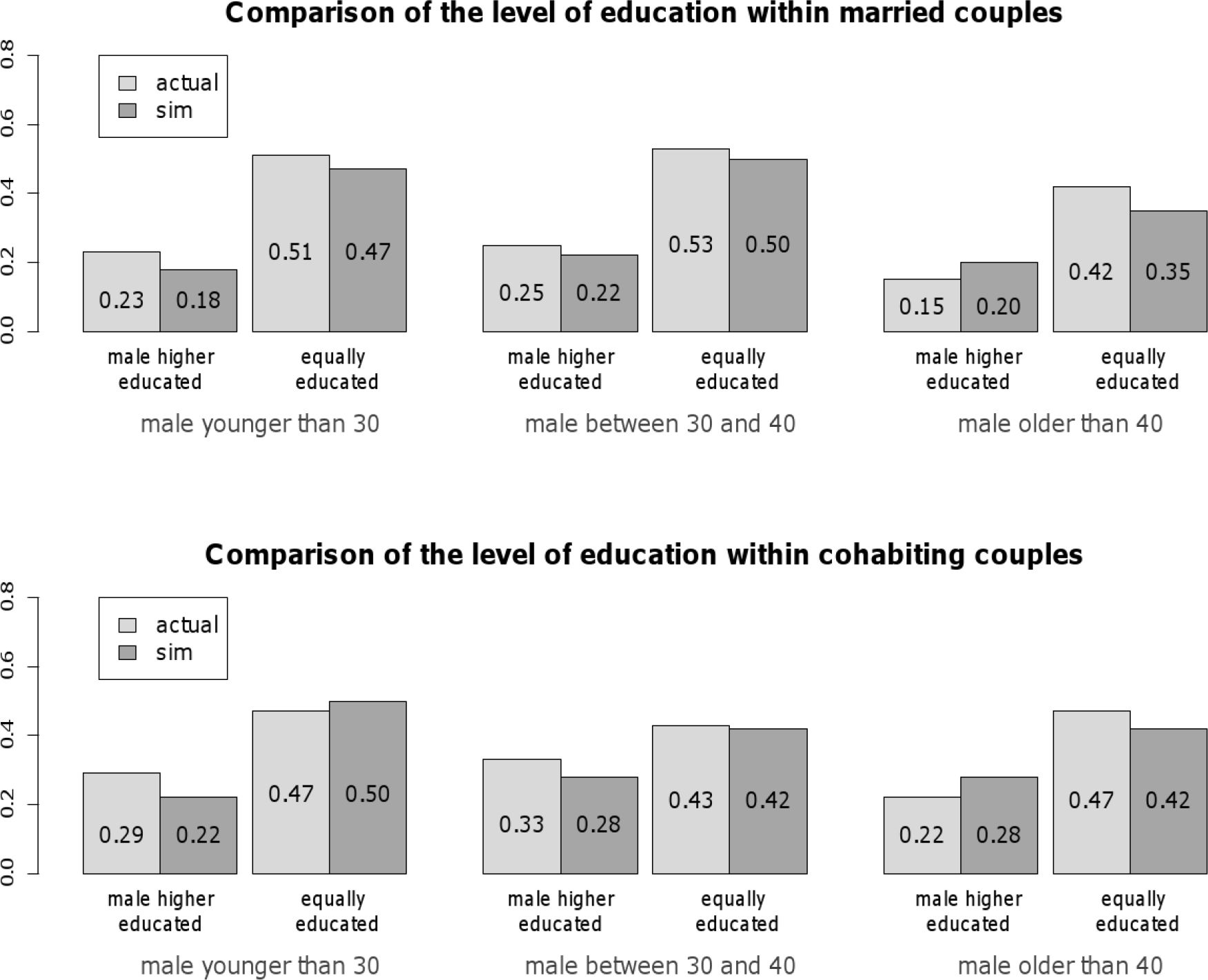
4.2.4 Comparison of attributes of actual and simulated couples
It is essential for the usefulness of the proposed mate-matching strategy that it resembles actual characteristics of partners in couples. Therefore, as a further validation step, the distribution of joint characteristics was analyzed, with a special emphasis on differences in educational attainment and age. The differences in the educational level of synthetic couples were compared to those of couples given in the NKPS (in the range from 1990 to 2002). Figure 8 contrasts simulated and actual data concerning the educational level within married couples (upper graph) and cohabiting couples (lower graph). Two types of couples are differentiated: couples in which the man is higher educated than the woman and couples in which both partners are equally educated. To account for eventual age effects, couples are additionally differentiated according to the man’s age at partnership onset: couples were considered where the man was younger than 30 years, couples where he was between 30 and 40 years old, and couples where he was older than 40 years. All presented numbers are given relative to the total number of couples in each age category. That is, the proportion of couples in which the woman is higher educated than the man can easily be derived by subtracting the numbers given for each age category from one. For married couples, comparing simulated and actual data shows a difference of maximal nine percentage points (in the category “couple in which the woman is higher educated than the man and the man has married younger than 30”). For cohabiting couples, the maximal difference between simulated and actual couples is seven percentage points (in the category “couple in which the woman is higher educated than the man and the man has married when he was between 30 and 40 years old”). overall, in the considered categorization the relative numbers of simulated and actual couples differ only slightly. This result shows that the simulation satisfactorily captures the overall pattern of differences in the educational level of spouses.

Differences in the educational level of spouses in observed and simulated couples. Each bar shows the percentage of females in the corresponding category.
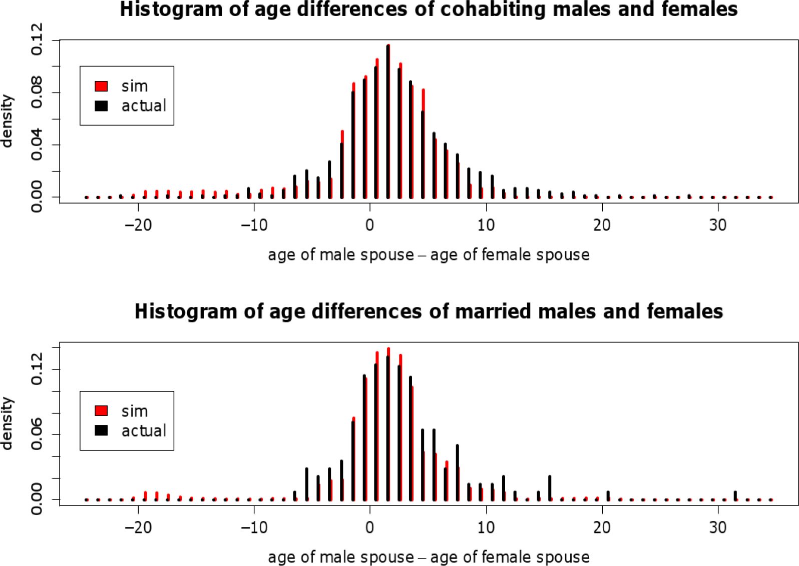
Age differences of spouses in observed and simulated couples.
Figure 9 depicts the distribution of age differences of cohabiting and married spouses (age of male minus age of female). The shapes of the simulated and actual frequency distributions, respectively, are very similar. Stochastic mate-matching algorithms that have so far been employed generally produce age difference distributions that are too flat (Leblanc et al., 2009). They are not capable of reproducing the observed peak at differences of [−1,1]. The proposed mate-matching algorithm is able to overcome this problem.
4.2.5 Handling situations of (relative) competition
A fundamental feature that demographers demand from a realistic mating model is the handling of (relative) competition (McFarland, 1972): an extra supply of single men of a certain age should decrease the number of paired men at all other ages (competition). The effect should be most pronounced at ages neighbouring the age group with the surplus of single men (relative competition). At the same time, the number of partnered women should increase over all ages. To check whether the present mate-matching procedure can handle such a situation, in the initial population the number of single men aged 27 was doubled. A comparison of the partnerships built under the initial and the modified setting shows that the proposed mate-matching procedures copes well when strong competition is present. In the cohort of men who turn 28 in 2004, an increased number of partnered men could be observed, but the number did not double as compared to the initial setting. Because of the surplus of younger rivals, the number of partnered men older than 28 declined. The effect is strongest in the neighbourhood of age 28 – which attests that the matching algorithm is able to handle situations of relative competition. For ages lower than 26, the number of partnered men is nearly identical to the initial setting. In this model the conditions, whether a female enters the partnership market or not, depends on her personal propensity and not on the availability of men. Therefore, even with a surplus of men in the mating pool, the number of partnered females remains stable.

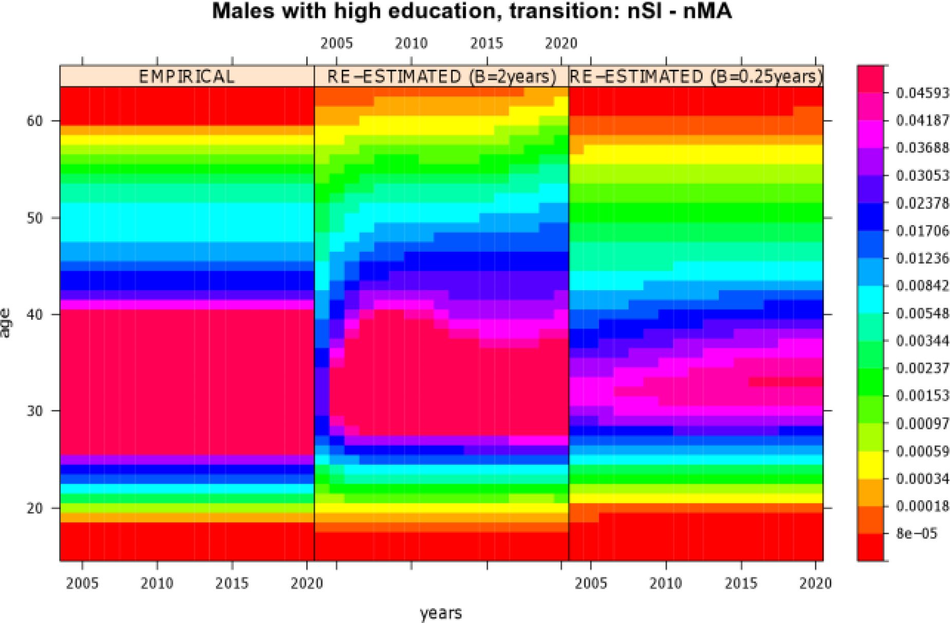
Comparison of re-estimated transition rates of highly educated males who experience a transition from “being single after leaving parental home” (nSI) to “married” (nMA). The left graph shows the empirical input rates used. The graph in the middle displays re-estimated rates from a simulation run with B = 2 years (intersection of the searching periods), and the right graph shows re-estimated rates from a simulation run with B = 0.25 years.
4.2.6 Sensitivity analysis of parameter values of algorithm
For the parameterization of the developed mate-matching algorithm specific values were proposed (cf. Table 1 on page 10). All parameter values were chosen deliberately. By means of sensitivity analysis their suitability was substantiated. In the following, the most important findings are discussed.
Setting the intersection of the searching periods (parameter B) to half a year was a compromise between finding enough potential partners in the market and not to be forced to strongly shift the event times that have been computed based on the microsimulation model. Testing different B values for showed that giving values bigger than half a year to B biased the simulation output regarding the timing of events more than setting to half a year. Choosing values smaller than half a year remarkably reduced the success probability of finding a proper spouse. As an example, for B = 2 years and for B = 0.25 years Figure 10 shows along empirical rates (left graph) re-estimated transition rates (graph in the middle and right graph) of highly educated males who experience a transition from “being single after leaving parental home” to “married”. Figure 10 is a level plot4 that presents rates along age and calendar time on a “rainbow” color scale. Compared to the empirical input rates, B = 2 years (graph in the middle) gave mating times significantly postponed in age and time. Especially, in the first year of simulation the proportion of mating events was significantly lower than indicated by the empirical input rates. In latter simulation years, the proportion of mate-matching events increased, partly following the pattern indicated by the empirical rates. For B = 0.25 years (right graph) the re-estimated rates were significantly lower than the empirical input rates, implying a large proportion of unsuccessful mate-seekers.
Decreasing the decrement δA of the aspiration level in case of rejection (in the original setting δA = 0.1) showed results similar to setting B to a value smaller than half a year: the chance to find an appropriate spouse in time decreased, and the simulation output was significantly biased. A small value of δA, like 0.01, meant that mate-seekers did not adequately adjust their aspiration according to the supply of potential spouses in the partnership market. Hence, mate-seekers were too “choosy”, and during simulation a large proportion of mate-seekers stayed unpaired. In contrast, setting δA to a relatively large value, like 0.5, caused mate-seekers who are not very discriminating regarding their conformance with potential spouses. As a consequence, simulated couple characteristics considerably differed from actual characteristics of partners in couples. For example, for δA = 0.5 the simulated distribution of age differences of cohabiting and married spouses were considerably flatter than the one of actual partners in couples (cf. Section 4.2.4).
Considering in the case study two percent of the Netherlands population meant a large enough proportion of a real population to assure that during simulation the pool of potential partners was mostly well filled. The situation that a seeker faced less than ten potential partners was reached infrequently. If aspiration levels were decremented because of “small pool size” (parameter δB, in the original setting δB = 0.3), then mostly in the initialization phase of simulation when the partnership market had been filled or when mature adults looked for a spouse (because they faced a reduced mating pool, cf. Section 4.2.3). For example, δB = 0.1 resulted in a slightly higher proportion of elderly people who stayed unpaired than δB = 0.3.
Decreasing the mean size μ of the upper bound of potential spouses that an individual can meet remarkably enlarges the pool of unsuccessful searchers. For example, for μ = 50 (in the original setting μ = 120) a surplus of almost ten percent individuals was found to remain unpaired in the partnership market. (The variability parameter σ of the pool size was set to 30.) Enlarging the mean size μ of the upper bound of potential spouses did not significantly affect the outcome of the mate-matching procedure, however, came at the expense of longer run times.
5. Discussion and outlook
In contrast to conventional population projection models, dynamic microsimulations are suitable to directly handle interactions between individuals, e.g., married couples (van Imhoff & Post, 1998). Modeling relations between spouses necessitates creating synthetic (married or cohabiting) couples, so an effective mate-matching procedure is needed. In this paper, the implementation of a technique to create synthetic couples, i.e., to match individuals, in a continuous-time microsimulation setting has been proposed and described.
For microsimulation models, two different approaches exist to handle the matching of spouses (see Section 2). In open models, an appropriate partner is created when needed. By contrast, in closed models an appropriate partner has to be found among the individuals of the model population. In terms of modeling and simulation, open models are straightforward; however, their interpretation is difficult. How can the appearance of a spouse be explained that was not present before? Closed models have a more plausible interpretation as marital matches are formed between individuals that already exist. Corresponding modeling and simulation approaches have to incorporate sophisticated matching algorithms that ensure the creation of synthetic marriages that follow a realistic pattern. Several suitable matching algorithms exist, but all of them apply to discrete-time models. No matching algorithm has so far been proposed for closed microsimulation models with a continuous-time scale. In discrete-time models, annual marriage markets are applied to create couples. This is a natural choice as in discrete-time models events are determined to occur in a given year. In continuous-time models by contrast, where events can occur at any point in time, annual marriage markets do not fit (see Section 3.2).
Therefore, in this paper it has been suggested to implement one partnership market that individuals can enter and leave over the complete simulation time range (cf. Section 3). In a continuous-time microsimulation, individual life courses are specified as sequences of waiting times to a next event. That is, the time point when individuals will experience the onset of a marriage or a cohabitation can be determined in advance. In the present mate-matching procedure, the waiting time until marriage or cohabitation onset is used for scanning potential partners. At the moment the simulation triggers for an individual as next event a marriage or a cohabitation event (i.e., when an individual’s wait for a partnership event starts), the individual enters a partnership market. Here, each “mating-minded” individual remains for a specific period of mate-searching and matching. In the market, the individual meets a limited number of potential partners at random. Each simulated individual exhibits a certain level of aspiration concerning attributes of potential spouses. To build synthetic couples, a decisionmaking process is simulated as to whether two individuals date each other by applying the individuals' aspiration levels and their mating probability. (Relying on the theory of assortative mating, pairs with similar attributes, like similar ages and educational levels, have a higher probability of mating.) A couple is formed if a positive decision has been made and the timing of the couple’s partnership formation events is consistent regarding their individual searching periods. Individuals that were inspected, but rejected, lower their level of aspiration accordingly. A marriage queue is used to implement the partnership market as basis for the matching procedure.
In order to illustrate the capability of the presented algorithm the MicMac microsimulation tool has been extended (Zinn et al., 2009). Using data from the Netherlands Kinship Panel Study (NKPS), logit models were estimated to quantify the likelihood of a union between potential pairings (see Section 4.2.1). The results were in accordance with common knowledge, e.g., among other aspects, the observation was made that people mate assortatively. Applying the estimated logit models as compatibility measure, simulations were run to project a synthetic population based on the population of the Netherlands (Section 4). To quantify marriage behavior micro-data from Statistics Netherlands were used. Population projections were conducted over 17 years, from 2004 to 2020.
To assess the quality of the proposed mate-matching technique, two validation steps were employed: first the empirical transition rates used as input were re-estimated from the simulation output (see Section 4.2.2). Then the distribution of joint characteristics in actual and simulated couples was analyzed (see Section 4.2.4).
The first strategy showed whether simplifying assumptions made during the mate-matching process caused biased simulation outcome. For example, slight changes to event times are allowed to form partnership onsets. Another, more severe problem arises in the case of unsuccessful searchers. If an individual is not able to find an appropriate partner during his/her searching period, currently his/her searching period is extended for half a year. A seeker might generally suffer from an exploited partner market, and his/her searching period is thus extended over and over again. Such shifts of event time mean ignoring already generated events and are in conflict with the stochastic model used for simulating life course events. In summary, empirical and re-estimated rates were not remarkably different. Consequently, the proposed mate-matching algorithm is suitable for successful incorporation into a continuous-time microsimulation.
In the second validation step, it was analyzed whether the attributes of simulated couples resemble the attributes of observed couples. The results showed that the proposed algorithm produces acceptable outcomes, e.g., it is capable of closely reproducing the distribution of the educational level of synthetic couples. Furthermore, the developed mate-matching algorithm copes with the challenge to reproduce the observed peak of the frequency distribution of age differences of spouses, an objective which other stochastic mate-matching algorithms failed to achieve (Leblanc et al., 2009).
Generally, a realistic mating model should be capable of handling situations of competition among mate searchers, i.e., an extra supply of single men of a certain age should decrease the number of paired men at all other ages (McFarland, 1972). Testing the developed mate-matching strategy to that effect showed that it is able to handle such situations (see Section 4.2.5).
For the developed algorithm a specific parameterization was proposed (cf. Table 1 on page 10). It was argued that for western European societies the chosen parametrization results in reasonable simulation outcome. To circumstantiate this argument a succinct sensitivity analysis was conducted, varying parameters (see Section 4.2.6). In particular, the length of the searching period was varied, the upper bound of the maximal number of potential spouses, the decrement of the individual aspiration level in case of rejection, and the decrement of the individual aspiration level in case of small pool size. In summary, for the considered case study, the sensitivity analysis confirms the feasibility of the chosen parametrization.
The mate-matching strategy presented in this paper can and will be extended. At the moment, individuals are matched based on actual preference patterns. However, preferences concerning the characteristics of a partner might change over calendar time, and such changes should be considered in the mate-matching process. Currently, the quality of a match has no effect on the stability of the union. However, the inclusion of quality seems natural. Furthermore, in the current model, individuals enter the partnership market based on empirical marriage rates or based on rates indicating cohabitation propensities. To correctly determine partnership events, however, instead of marriage or cohabitation rates, rates indicating the willingness to mate would have to be used. One way to obtain those rates would be to hypothesize them based on external knowledge of the phenomenon. Pairing individuals generally raises problems concerning the modeling and simulation of linked lives. An abstract DEVS (Discrete Event Specification Language)-based model to establish and simulate linked lives in continuous-time is currently under examination.
Footnotes
1.
Author’s current affiliation: University of Bamberg, National Educational Panel Study, Bamberg, Germany.
2.
That is, the length of the searching period is determined exogenously. In doing so, an approach proposed by Billari (2000) is adopted. However, as opposed to Billari (2000) heterogeneity in the length of the searching period is not considered explicitly.
3.
4.
A level plot is a type of graph that displays on a colored surface three dimensional data points. Different colors map different valued data points. Commonly, abscissa and ordinate correspond to time or geographical dimensions. A level plot is an alternative to a contour plot.
References
-
1
APPSIM - modelling family formation and dissolution. Working Paper 4, NATSEM, National Center for Social and Economic ModellingAPPSIM - modelling family formation and dissolution. Working Paper 4, NATSEM, National Center for Social and Economic Modelling, University of Canberra.
-
2
Channels of social influence on reproductionPopulation Research and Policy Review of Economics and Statistics 22:527–555.
-
3
Searching for mates using ‘fast and frugal heuristics: A demographic perspectiveIn: G Ballot, G Weisbuch, editors. Applications of Simulation to Social Sciences. Oxford: Hermes Science Publications. pp. 53–65.
-
4
Who Marries Whom? Educational Systems as Marriage Markets in Modern Societies331–342, Assortative mating in cross-national comparison: A summary of results and conclusions, Who Marries Whom? Educational Systems as Marriage Markets in Modern Societies, Dordrecht, Kluwer.
-
5
Matchmaker, matchmaker, make me a matchBrazilian Electronic Journal of Economics, 4, 2.
- 6
-
7
MortalitySmooth: Smoothing Poisson counts with P-splinesMortalitySmooth: Smoothing Poisson counts with P-splines, R package version 1.0, MPI Rostock, http://CRAN.R-project.org/package=MortalitySmooth, [accessed November 2011].
-
8
Generalized linear array models with applications to multidimensional smoothingJournal of the Royal Statistical Society 68:259–280.
-
9
On a least square adjustment of a sampled frequency table when the expected marginal totals are knownAnnals of Mathematical Statistics 11:427.
-
10
Codebook of the Netherlands Kinship Panel Study: A multiactor, multi-method panel study on solidarity in family relationships, wave 1. NKPS Working Paper 4, NIDICodebook of the Netherlands Kinship Panel Study: A multiactor, multi-method panel study on solidarity in family relationships, wave 1. NKPS Working Paper 4, NIDI, The Hague.
-
11
Handbook of the Life Course3–19, The emergence and development of life course theory, Handbook of the Life Course, Handbooks of sociology and social research, Springer.
-
12
KAMA: A temperature-driven model of mate-choice using dynamic partner representationsAdaptive Behaviour 16:71–95.
-
13
College admissions and the stability of marriageThe American Mathematical Monthly 69:9–9.
-
14
Discrete-time and continuous-time approaches to dynamic microsimulation (reconsidered). Technical report, NATSEM, National Center for Social and Economic Modelling, University of CanberraDiscrete-time and continuous-time approaches to dynamic microsimulation (reconsidered). Technical report, NATSEM, National Center for Social and Economic Modelling, University of Canberra, University of Canberra.
-
15
Description of the microsimulation model. Technical report, MicMac project, MPIDRDescription of the microsimulation model. Technical report, MicMac project, MPIDR, Rostock.
-
16
Report on projections by the level of education (future human capital: Estimates and projections of education transition probabilities). Technical report, MicMac project, Vienna Institute of Demography, Austrian Academy of SciencesReport on projections by the level of education (future human capital: Estimates and projections of education transition probabilities). Technical report, MicMac project, Vienna Institute of Demography, Austrian Academy of Sciences.
-
17
The SOCSIM demographic-sociological microsimulation program: Operating manual, Institute of International Studies, University of California, Berkeley, Research Series, No. 27The SOCSIM demographic-sociological microsimulation program: Operating manual, Institute of International Studies, University of California, Berkeley, Research Series, No. 27.
-
18
SOCSIM II: A sociodemographic microsimulation program rev. 1.0: Operating manualRegents of the University of California.
- 19
- 20
-
21
Age profiles estimation for family and fertility events based on micro data: The MAPLE (method for age profile longitudinal estimation)In Joint Eurostat /UNECE Work Sessions on Demographic Projections.
-
22
Intermarriage and homogamy: Causes, patterns, trendsAnnual Review of Sociology 24:395–421.
-
23
Statistical inference in the Lexis diagramPhilosophical Transactions of the Royal Society of London: Physical Sciences and Engineering 332:487–487.
-
24
Australia’s microsimulation model - DYNAMOD. Technical report, NATSEM, National Center for Social and Economic Modelling, University of CanberraAustralia’s microsimulation model - DYNAMOD. Technical report, NATSEM, National Center for Social and Economic Modelling, University of Canberra.
- 25
-
26
A match made in silicon: Marriage matching algorithms for dynamic microsimulationpaper presented at the 2nd general conference of the International Microsimulation Association, Ottawa.
-
27
Comparison of alternative marriage modelsIn: T Greville, editors. Population Dynamics. New York: Academic Press. pp. 89–106.
-
28
project hompageproject hompage, www.micmac-projections.org>, [accessed November 2011].
-
29
Withholding age as putative deception in mate search tacticsEvolution and Human Behavior 20:53–53.
-
30
Mate matching for microsimulation models. Technical Paper 3, Long-Term Modeling Group, Congressional Budget OfficeMate matching for microsimulation models. Technical Paper 3, Long-Term Modeling Group, Congressional Budget Office, Washington, DC.
- 31
-
32
Confession of a microsimulator: Problems in modeling the demographic kinshipHistorical Methods 26:161–161.
-
33
Parallel discrete-event simulation of population dynamicsIn: SJ Mason, RR Hill, L Mönch, O Rose, T Jefferson, JW Fowler, editors. Proceedings of the 2008 Winter Simulation Conference. Piscataway, New Jersey: Institute of Electrical and Electronics Engineers, Inc. pp. 1047–1054.
- 34
-
35
Aggregate age-at-marriage patterns from individual mate-search heuristicsDemography 42:559–574.
-
36
Sexual selection and the descent of man, 1871–1971In: B Campbell, editors. Parental Investment and Sexual Selection. Chicago: Aldine. pp. 136–179.
-
37
Microsimulation methods for population projectionPopulation: An English Selection, New Methodological Approaches in Social Sciences 10:97–138.
-
38
2030’s seniors: Kin and step-kin. Technical report, University of California2030’s seniors: Kin and step-kin. Technical report, University of California, Berkeley.
-
39
New Frontiers in Microsimulation ModellingSurrey353–376, Continuous-time microsimulation in longitudinal analysis, Farnham (UK), Ashgate, Book released during 2nd International Microsimulation Conference, Ottawa, June 2009.
-
40
The role of microsimulation in longitudinal data analysisSpecial Issue on Longitudinal Methodology, Canadian Studies in Population 28:313–313.
-
41
Proceedings of the 2009 Winter Simulation ConferenceMic-core: A tool for microsimulation, Piscataway (NJ), IEEE.
Article and author information
Author details
Acknowledgements
This work is a result of the MicMac project. The Centraal Bureau voor de Statistiek in the Netherlands provided data from the Fertility and Family Survey for the Netherlands. The Netherlands Kinship Panel Study is funded by grant 480-10-009 from the Major Investments Fund of the Netherlands Organization for Scientific Research (NWO), and by the Netherlands Interdisciplinary Demographic Institute (NIDI), Utrecht University, the University of Amsterdam, and Tilburg University. This paper would never have been written without the help of several persons: Particular thanks go to Jutta Gampe for her fruitful supervision. Adelinde Uhrmacher and Frans Willekens volunteered to read several versions of the paper, and their comments significantly improved the quality of the paper. The input data files for the microsimulation example were prepared by Ekaterina Ogurtsova. Jim Oeppen helped with general advice. Basic ideas of mate-matching in continuous time go back to discussions with Jan Himmelspach and Frans Willekens. Nico Keilman provided very helpful comments on the last draft version of this paper.
Publication history
- Version of Record published: June 30, 2012 (version 1)
Copyright
© 2012, Zinn
This article is distributed under the terms of the Creative Commons Attribution License, which permits unrestricted use and redistribution provided that the original author and source are credited.